“Sampling vs analytical error: where the money is …”

Along the full lot-to-analysis pathway

Analytical measurements comprise at least two error generating steps: deline­ating and extracting the primary sample, and analysis of the analytical aliquot. There may be several sub-sampling steps before having a sufficiently small aliquot (analytical sample) of the original mate­rial ready for proper analysis. In this chain of operations, the weakest link determines how reliable the analytical result is. The reason is that variances (squared standard deviations) are additive.

If only one primary sample is processed through i stages, the error vari­ance of the analytical result, a_L is:

\[s_{a_{L}}^{2} = \sum_{i=1}^{I}s_{i}^{2} \]

This variance can be reduced (always popular for those who worry about the total sampling-plus-analy­sis error) by taking replicate samples at different stages. Consider a three-level process: n₁ primary samples are extracted from the lot, with each primary sample processed and divided into n₂ secondary samples—of which nlab analytical samples are finally anal­ysed. In this case Equation 2 shows how the complement of stage error variance components propagate to the analytical result.

\[s_{a_{L}}^{2} = {s_{1^{}}^{2} \over n_{1}} + {s_{2^{}}^{2} \over n_{1} \bullet n_{2} } + {s_{lab^{}}^{2} \over n_{1} \bullet n_{2} \bullet n_{lab} }\]

The total number of samples analysed is n_tot = n₁ • n₂ • n_lab.

From a replication design, the vari­ance components s_i ² can be estimated by using the statistical facility of analysis of variance (ANOVA), or analysis of rela­tive variances (RELANOVA).^₁

Master example: the effectiveness of replication

The following example will help gain insight into where efforts to reduce and control the total accumulated error is best spent. Let us consider three schemes where, for each scheme, the relative standard deviation error estimates are: sr1 = 10 %, sr2 = 4 % and sr2 = 2 %.

A) No replicates, n₁ = n₂ = n_lab = 1. Total number of samples analysed is 1.

\[s_{a_{L}}^{2} = (10\%)^{2} + (4\%)^{2} + (2\%)^{2} ) = 120(\%)^{2} \text{and} s_{a_{L}} = 11.0\%\]

B) Primary samples replicated, n₁ = 10; n₂ = n_lab = 1. Total number of samples analysed is 10.

\[s_{a_{L}}^{2} = {(10\%)^{2} \over 10} + {(4\%)^{2} \over 10} + {(2\%)^{2} \over 10} = 12.0(\%)^{2} \text{and} s_{a_{L}} = 3.5\%\]

C) Primary samples and duplicated analytical samples, n₁ = 5; n₂ = 1; n_lab = 2. Total number of samples analysed is again 10.

\[s_{a_{L}}^{2} = {(10\%)^{2} \over 5} + {(4\%)^{2} \over 5\bullet 1} + {(2\%)^{2} \over 5\bullet 1\bullet 2} = 23.6(\%)^{2} \text{and} s_{a_{L}} = 4.9\%\]

This example demonstrates that even if the best and most expensive analyti­cal technology available is used in the laboratory, this does not by itself guaran­tee a reliable result with minimised total uncertainty. Still, some laboratories routinely run analyses in duplicates or even in triplicates to be sure that their results are “correct”. While analytical costs have doubled or tripled, noth­ing is gained! It is also common that the uncertainty estimates which laboratories assign to their results are based on the results of the laboratory replicates only; in reality hiding the full pathway uncer­tainty.

Selection of optimal sampling mode

Most current standards and guidelines assume glibly—although very rarely expressed explicitly—that sampling errors can be estimated using standard statis­tics. This is based on another assumption, that of a random spatial analyte distribu­tion within the sampling target. When primary samples are extracted from large lots like process streams, environ­mental targets, shipment of raw materials or commodities or from manufactured products, the same assumption of “normality” may in fact lead to sampling plans that are more expensive than the optimised plan and, more importantly, do not provide reliable results. When the purpose of sampling is to estimate the mean value of the lot, the first issue to address is which sampling mode to use: random, stratified or systematic. Figure 1 shows and compares the principle of these modes. Very few guidelines refer to the sampling modes at all. Very often in monitoring programmes samples are collected systematically (all good), but the resulting analytical results are then treated as so-called random data sets. As the following example shows this actu­ally results in a massive loss of informa­tion.

Figure 1 presents a comparison of these three fundamental sampling modes as applied to a process steam.

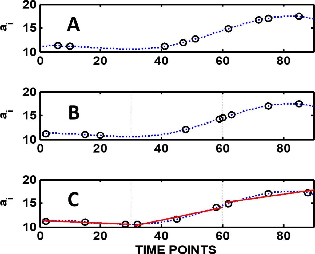
First, there is no significant difference between them if the process standard deviation is estimated from all nine samples taken in each mode, i.e. the nine samples are treated as one data set. But their difference becomes clear when the mean of the whole process range is calculated. The bias of the mean is decreased from 4.49 % (random) to 3.92 % (stratified) and to –0.48 % (systematic) and the relative standard deviation of the mean from 11.3 % (random) to 8.28 % and to 2.26 %. The difference is even more clear if, based on these data, a sampling plan is requested, for example, with a target that the relative standard deviation of the mean shall not exceed 1 %. The “expert” who recom­mends random sampling gives a plan that requires extraction of no less than 385 samples. However, a stratified sampling plan will only require 186 samples—whereas if the systematic mode is selected, only 12 samples are needed to reach the relative standard deviation target. To summarise, in cost– benefit analysis of an analytical sampling plan the selection mode is crucial. To select the optimal sampling mode and number of replicates, the unit costs are needed. Operators usually can esti­mate the cost structure, but the variance estimates can seldom be estimated theo­retically. Sometimes they can be esti­mated from the existing data, but very often pilot studies are needed. Combining specific variance estimates with unit costs of the various operations in the full analytical measurement pathway will allow drastic improvements in the efforts needed; some examples are given below. Further examples of the informed use of the Theory of Sampling (TOS)’ principles in the context of total expenditure estima­tion are given in Reference 2.

The value of engaging in proper sampling

Case 1

A pulp mill was extracting a valuable side product (b-sitosterol) which is used in the cosmetic and medical industries, and which has high quality require­ment. Customers requested a report on the quality control system from the company in question. I was asked to audit the sampling and analytical proce­dures and to give recommendations, if needed. I proposed some pilot studies to be carried out and based on these empirical results recommended a new sampling system to be implemented— this was accepted.

In comparison to the old, the new sampling system annually saved the equivalent of one laboratory techni­cian’s salary.

Case 2

An undisclosed pulp mill was feeding a paper mill through a pipeline pump­ing the pulp at about 2 % “consistency” (industry term for “solids content”). The total mass of the delivered pulp was estimated based on the measurements with a process analyser installed in the pipeline immediately after the slurry pump at the pulp factory. The receiv­ing paper mill claimed that it could not produce the expected tonnage of paper from the tonnage of pulp they had been charged for by the pulp factory. An expert panel was asked to check and evalu­ate the measurement system involved. A careful audit, complemented with TOS-compatible experiments, revealed that the consistency measurements were biased, in fact giving up to 10 % too high results. The bias was found to originate from two main sources. 1) The process analyser was placed in the wrong loca­tion and suffered from a serious incre­ment delimitation error; this is an often-met weakness of process analysers installed on or in pipelines. 2) The other error source was traced to the process analyser calibration. It turned out that the calibration was dependent on the qual­ity of the pulp: softwood and hardwood pulps needed different calibrations. By a determined effort to make the process sampling system fully TOS-compatible, and by updating the analyser calibration models, it was possible to fully eliminate the 10 % bias detected.

It is interesting to consider the payback time for the efforts involved to focus on proper TOS in this case. The pulp produc­tion rate was about 100,000 ton y^–1, or 12 ton h^–1. The contemporary price of pulp could be set as an average of $700 ton^–1, so the value produced per hour was approximately $8400 h^–1. The value of the 10 % bias would thus be $840 h^–1 ($7 million y^–1). As the cost of the evaluation study was about $10,000 the payback time of the audit and the panel investigations was about 12 h.

It does not have to be expensive to invoke proper TOS competency—it is often possible to get a better quality at lower cost.

Are our current sampling standards and guides adequate?

In most current standards, the findings of the TOS have often been ignored, or at best only partially recommended. Statistical considerations assume that sampling errors can be estimated using classical statistics which are based on the ubiquitous assumption of random spatial analyte distributions within the sampling targets. The basic three sampling modes, random, stratified or system­atic, are seldom even mentioned as options. As shown above, when primary samples are taken from large lots like process streams, environmental targets, shipment of raw materials or products, ill-informed or wrong assumptions simply lead to wrong conclusions, and usually too expensive or inefficient solutions. More examples are given below.

Case 3: Estimation of the concentration genetically modified (GMO) soybeans

In the European Union, the limit of acceptable GMO content in soybeans is 1 % (or 1 GMO bean/100 beans). If the content exceeds this limit, the lot must be labelled as containing GMO material. To allow for the sampling and analyti­cal error, in practice 0.09 % is used as the effective threshold limit for deciding on labelling the material as containing GMO or not. Theoretically, this seems a simple sampling and analysis problem. GMO soybeans and their natural coun­terparts are identical with no tendency to segregate. So, theoretically the required sample size can be estimated from considerations assuming a binomial distribution. The reality is very different, however.

In References 3–5 experimental analytical data from the KeLDA project were re-analysed, with a special focus on the inherent sampling issues involved. In the KeLDA project, 100 shiploads arriving at different EU ports were sampled by collecting 100 primary 0.5-kg samples (each containing approximately 3000 beans) using systematic sampling. At the 1 % concentration level, the relative standard deviation of the total analytical error (s_TAE) was found to be 11.4 %. For an ideal binomial mixture, conventional statistical calculations showed that the minimum number of 0.5-kg samples to be analysed in order to guarantee that the probability (risk) is less than 5 % that the mean 0.09 % could be from a lot having mean concentration above 1 %— is 10 samples. The official number of samples recommended by many organ­isations vary between 4 and 12. So far, so good… if the conventional assump­tions hold up to reality… alas!

A shipload often consists of prod­ucts from many different sources having different GMO concentrations. In such cases the lot can be seriously segregated in the distributional sense w.r.t. domains having different GMO contents, making the assumption of spatial randomness grossly erroneous. Instead of the theo­retical 10 samples, the thorough study reported in Reference 4 (lots of statis­tics in there, but they are not neces­sary for the present purpose) ended up with a much higher required number of samples needed, 42 to be precise (a famous number, if the reader is fan of Douglas Adams’ Hitchhiker’s Guide to the Universe). It is this number of samples which must be collected using the systematic sampling mode to make a correct decision regarding the labelling issue.

From enclosed stationary lots, such as the cargo hold(s) of grain shipments, or truckloads, railroad cars, silos, storage containers… it is in general impossible to collect representative samples without a TOS intervention. Samples must be taken either during Ioading or during unloading of the cargo, i.e. when the cargo lot is in a moving lot configuration on a conveyor belt. Otherwise, the average concentra­tion simply cannot be reliably estimated. References 3–5 tell the full story, the conclusion of which is: conventional statis­tics based on the assumption of spatial random analyte distributions always runs a significant risk of underestimating the number of samples needed to reach a specified quality specification—compared to informed TOS-competent understand­ing of heterogeneity, spatial heterogeneity in this case. Proper TOS-competence is a must.

Case 4: Sampling for aflatoxins in peanut kernels

Mycotoxins, e.g. aflatoxins and ochratox­ins, are poisonous and are also regarded as potent carcinogens. Their contents in foodstuff must, therefore, be care­fully monitored and controlled and the levels regarded safety are extremely low, down to 5 mg kg^–1 (ppm), or even lower. But detection and quantifica­tion even of these very low concentra­tion levels is usually not a challenge for modern analytical techniques in dedi­cated analytical laboratories. The real challenge is how to provide a guaran­teed representative analytical aliquot (of the order of grams only) from the type of large commercial lots used in the inter­national trade of such commodities (of the order of magnitude of thousands of tons). Effective sampling ratios are staggering, e.g. 1 : 106 to 1 : 109, or even higher. It is somebody’s responsibility that the overwhelming 1 / 106 to 1 / 109 mass reduction is scrupulously repre­sentative at/over all sampling and sub-sampling stages. It is fair to say, that this setup is not always known, recognised, far less honoured in a proper way, sadly (because this is where the money is lost, big time) with the unavoidable result that nobody (nor any guideline or standard) can guarantee representativity.

Campbell et al.⁶ carried out an exten­sive sampling study in connection with analysing peanuts for aflatoxins. It is interesting to study their findings using the principles of TOS: they sampled a lot having an average aflatoxin content 0.02 mg kg^–1 by taking 21.8 kg primary samples. The average aflatoxin content of individual “mouldy” peanut kernels was 112 mg kg^–1. The average mass of one peanut kernel is about 0.6 g. In Reference 6 it was found that the experimental rela­tive standard deviation of the 21.8-kg primary samples sr(exp) was 0.55 = 55 %. This empirical result is below the theoreti­cally expected value, however, indicating that “something” is not right … A TOS rationale follows below.

Involving TOS

The mass of aflatoxin in a single mould contaminated kernel: m_a = 112 mg kg^–1 × 0.6 × 10^–3 kg = 0.0672 mg. If the acceptable average aflatoxin level is 0.02 mg kg^–1, this result means that just one mouldy peanut is enough to contaminate a whole sample of 3.36 kg. On the other hand, if the maximum tolerable level is only 0.005 mg kg^–1, one kernel will contaminate a 13.44- kg sample. If the kernels are crushed to 50 mg fragments, average samples containing one contaminated fragment are now 0.28 kg and 1.12 kg at average aflatoxin concentrations 0.02 mg kg^–1 and 0.005 mg kg^–1, respectively. The relative standard deviation of a sample contain­ing one contaminated peanut taken from a random distribution is 1 = 100 %.

The theoretical relative standard deviation of a 21.8-kg sample from a random mixture is s_r = 39.3 % whereas the experimental value was 55 %. The difference between these variance esti­mates [0.552 – 0.3932 = 0.148, or 38.5 % as RSD %] is a strong indication of spatial segregation. Such segregation of myco­toxins in large lots is a natural phenom­enon, since moulds, which are producing the toxins, tend to grow in localised “pockets” where mould growth condi­tions are favourable. As an unavoidable consequence, the distribution of contam­inated individual nuts within the full lot volume is in reality far from random. Because large lots, almost exclusively found in restricted and confined contain­ers, cannot be well mixed (randomised), segregation has a drastic adverse effect on sampling uncertainty at the primary sampling stage—whereas at all later sample preparation stages, when only small masses are handled, it is possible to randomise various sized sub-samples by careful mixing, and here the theoreti­cal values can be used to estimate the uncertainty of the sub-sampling steps involved.

For the ideal case of truly random mixtures, it is easy to estimate the sample size that gives the required relative stan­dard deviation of the lot as a function of the primary sample size. For the two lot averages used here as examples, aL is 0.02 mg kg^–1 and 0.005 mg kg^–1, and targeting to 10 % relative standard devia­tion of the lot mean, the realistic mini­mum sample sizes are:

\[m_{s} = {(100\%)^{2} \over (10\%)^{2}}3.36kg = 336kg \\
m_{s} = {(100\%)^{2} \over (10\%)^{2}}13.44kg = 1344kg\]

If the distribution is indeed random, the m_s can be a composite sample or single increment, the expected RSD of the mean is the same, 10 %, indepen­dent of the sampling mode. But the situation is radically different if there is indeed segregation, e.g. clustering of the contaminated peanuts. Then the required primary sample size and number will depend on the spatial distribution pattern and this can only be estimated empirically, either by a variographic experiment or by involv­ing an ANOVA design, see References 3–6.

The only result that can be estimated from the reported data in the Campbell et al. study, is how many 21.8-kg samples, nreq, are needed if random sampling is used. If the target threshold is 10 % RSD of the mean at aL = 0.02 mg kg^–1:

\[n_{s(req)} = {s_{r(exp))}^{2} \over (10\%)^{2} } = {(55\%)^{2} \over (10\%)^{2} } = 30.3\]

and the total mass of the samples 30.3 • 21.8 kg ≈ 660 kg.

Implications for commodity trade a.o.

In international trade agreements regard­ing foodstuffs, the tight limits set by regulators must be met at the entry port before the cargo materials can be released to the markets. As the examples above show, sampling and sample prep­aration for analysis are extremely difficult when the unwanted contaminants are present at their usual low, or very low ppm (or even ppb) levels. In the case of the present peanut example, at an aver­age concentration 5 μg kg^–1 in an ideal case (i.e., assuming randomness), the weight of the total number of primary samples should be about 1350 kg if the if 10 % relative standard deviation is the target. In sample preparation, if the secondary samples are each 10 kg and the analytical sample from which the toxins are extracted, are, say, 200 g, the peanuts must be ground to 0.45 mg and 0.09 mg particle sizes corresponding to approximately 0.96 mm and 0.56 mm particle diameters. But these are the results of an ideal case, very rarely found. Segregation makes the theoretical considerations much more complicated.

The simple moral from underlying complexities

The above technical intricacies notwith­standing, it is abundantly clear, that the quality of sensitive foodstuffs must be adequately monitored—and it is equally clear that at the inherent trace and ultra-trace levels of the analytes involved, the primary sampling and sample prepara­tion are extremely difficult operations, but absolutely necessary! If the uncer­tainties of the analytical results are too high, this means that a high number of shipments containing excess amount of the contaminants may enter the market essentially undetected and, vice versa, shipments containing acceptable mate­rial may be stopped—but both types of misclassification are not caused by analytical difficulties. The resulting economic losses are huge, for each ship­load that is wrongly stopped and retuned due to “erroneous” analytical results. The lesson from the somewhat technical story above is clear: primary sampling, and subsequent sub-sampling and sample preparation errors, are very nearly always the real culprits—perpe­trators are not to be found in analyti­cal laboratories.

What to do?

When decision limits are set, the capa­bility of modern analytical instruments alone cannot be used as the guide for reliability. The capability of the whole measurement chain must be evalu­ated. If it turns out that the proposed decision limit is so low that it cannot be achieved at acceptable costs, even when the best methods of the TOS are applied in designing the sampling and measure­ment plan, then it must be decided what are the maximum allowable costs of the control measurements. First, then is it possible to set realistic decision limits so that they can be reached with methods optimised to minimise the uncertainty of the full lot-to-aliquot measurement pathway within a given budget which is regarded as acceptable; a more fully developed treatment of these interlinked technical and economic factors can be found in References 1 and 2.

References

[1] P. Minkkinen, “Cost-effective estimation and monitoring of the uncertainty of chemical measurements”, Proceedings of the Ninth World Conference on Sampling and Blending, Beijing, China, pp. 672–685 (2019).
[2] P. Minkkinen, “Practical applications of sampling theory”, Chemometr. Intell. Lab. Syst. 74, 85–94 (2004). https://doi.org/10.1016/j.chemolab.2004.03.013
[3] K.H. Esbensen, C. Paoletti and P. Minkkinen, “Representative sampling of large kernel lots I. Application to soybean sampling for GMO control”, Trends Anal. Chem. 32, 154–164 (2012). https://doi.org/10.1016/j.trac.2011.09.008
[4] P. Minkkinen, K.H. Esbensen and C. Paoletti, “Representative sampling of large kernel lots II. Theory of sampling and variographic analysis”, Trends Anal. Chem. 32, 165–177 (2012). https://doi.org/10.1016/j.trac.2011.12.001
[5] K.H. Esbensen, C. Paoletti and P. Minkkinen, “Representative sampling of large kernel lots III. General considerations on sampling heterogeneous foods”, Trends Anal. Chem. 32, 178–184 (2012). https://doi.org/10.1016/j.trac.2011.12.002
[6] A.D. Campbell, T.B. Whitaker, A.E. Pohland, J.W. Dickens and D.L. Park, “Sampling, sample preparation, and sampling plans for foodstuffs for mycotoxin analysis”, Pure Appl. Chem. 58(2), 305–314 (1986). https://doi.org/10.1351/pac198658020305
Glossary
A B C D E F G H I J K L M N O P Q R S T U V W X Y Z
A
Aliquot
An aliquot is the ultimate sub-sample extracted in a 'Lot-to-Aliquot' pathway for analysis. By analogy, process analytical technology involves the extraction of virtual samples, which are defined volumes of matter interacting with a process analytical instrument.
Analysis
Analysis is the systematic examination and evaluation of the ultimate sub-sample of chemical, biological, or physical substance (Aliquot) to determine its composition, structure, properties, or presence of specific components.
Analytical Bias
Analytical bias is a systematic deviation of measured values from true values.  An analytical bias can arise from multiple sources, including instrument calibration errors, sample preparation techniques, operator method, or inherent methodological limitations. Unlike random errors, which fluctuate unpredictably, analytical bias consistently skews results in a particular direction. Identifying and correcting this bias is crucial to ensure the accuracy and reliability of analytical data (bias correction).
Analytical Precision
Analytical precision refers to the degree of agreement among repeated analyses of the same aliquot under identical conditions. It reflects the consistency and reproducibility of the results obtained by a given analytical method. High precision indicates minimal random analytical error and close clustering of analytical results around an average. Precision does not necessarily imply accuracy, as a method can be precise yet still yield systematically biased results.
C
Composite Sampling
Composite sampling extracts a number (Q) of  Increments, established to capture the Lot Heterogeneity. Composite sampling is the only way to represent heterogeneous material. A composite sample is made by aggregating the Q increments subject to the Fundamental Sampling Principle (FSP). The required amount of increments for the requested Representativity Q can be carefully established to make sampling fit-for-purpose.
Compositional Heterogeneity (CH)
Compositional heterogeneity is the variation between individual fundamental units of a target material (particles, fragments, cells, ...). CH is an intrinsic characteristic of the target material to be sampled.
Correct Sampling Errors (CSE)
CSE are the errors that cannot be eliminated even when sampling correctly (unbiased) according to the Theory of Sampling (TOS). CSE are caused by Lot Heterogeneity and can only be minimised.
There are two Correct Sampling Errors (CSE):
1. Fundamental Sampling Error (FSE)
2. Grouping and Segregation Error (GSE)
Crushing
Crushing is the term used for the process of reducing particle size. Other terms are grinding, milling, maceration, comminution. Particle size reduction changes the Compositional Heterogeneity (CH) of a material. Composite Sampling and crushing are the only agents with which to reduce the Fundamental Sampling Error (FSE).
D
Data Format
Data must be reported as the measurement results and the Measurement Uncertainties stemming from sampling and analysis. Note that MUAnalysis and MUSampling are expressed as variances.
Data =            Measurement +/- (MUSampling ; MUAnalysis)
Example:       375 ppm +/- (85 ppm ; 18 ppm)
Note that the Uncertainties 85 ppm and 18 ppm are the square roots of MUSampling and MUAnalysis.
Data Uncertainty
Distributional Heterogeneity (DH)
Distributional heterogeneity is the variation between groups of fundamental units of a target material. Groups of units manifest themselves as Increments used in sampling. DH is an expression of the spatial heterogeneity of a material to be sampled (Lot).
DS3077:2024
This standard is a matrix-independent standard for representative sampling, published by the Danish Standards Foundation. This standard sets out a minimum competence basis for reliable planning, performance and assessment of existing or new sampling procedures with respect to representativity. This standard invalidates grab sampling and other incorrect sampling operations, by requiring conformance with a universal set of six Governing Principles and five Sampling Unit Operations. This standard is based on the Theory of Sampling (TOS).
webshop.ds.dk/en/standard/M374267/ds-3077-2024
Dynamic Lot
A dynamic lot is a moving material stream where sampling is carried out at a fixed location. For both Stationary Lots and Dynamic Lots, sampling procedures must be able to represent the entire lot volume guided by the Fundamental Sampling Principle.
F
Fractionation
Fractionation is a way of processing a Lot or Sample before sampling (or subsampling). Fractionation separates materials/lots into fractions according to particle properties, e.g. size, density, shape, magnetic susceptibility, wettability, conductivity, intrinsic, or introduced moisture ...
Fundamental Sampling Error (FSE)
FSE results from the impossibility to fully compensate for inherent Compositional Heterogeneity (CH) when sampling. FSE is always present in all sampling operations but can be reduced by adherence to TOS' principles. Even a fully representative, non-biased sampling process will be unable to materialise two samples with identical composition due to Lot Heterogeneity. FSE can only be reduced by Crushing (followed by Mixing / Blending) i.e. by transforming into a different material system with smaller particle sizes.
Fundamental Sampling Principle (FSP)
The Fundamental Sampling Principle (FSP) stipulates that all potential Lot Increments must have the same probability of being extracted to be aggregated as a Composite Sample. Sampling processes in which certain areas, volumes, parts of a Lot are not physically accessible cannot ensure Representativity.
G
Global Estimation Error (GEE)
The GEE is the total data estimation error, the sum of the Total Sampling Error (TSE) and the Total Analytical Error (TAE).
Governing Principles
Six Governing Principles (GP) describe how to conduct representative sampling of heterogeneous materials:
1) Fundamental Sampling Principle (FSP)
2) Sampling Scale Invariance (SCI)
3) Principle of Sampling Correctness (PSC)
4) Principle of Sampling Simplicity (PSS)
5) Lot Dimensionality Transformation (LDT), and
6) Lot Heterogeneity Characterisation (LHC).
Grab Sampling
Process of extracting a singular portion of the Lot. Grab sampling cannot ensure Representativity for heterogeneous materials. Grab sampling results in a sample designated a Specimen.
Grouping and Segregation Error (GSE)
The GSE originates from the inherent tendency of Lot particles, or fragments hereof, to segregate and/or to group together locally to varying degrees within the full lot volume. This spatial irregularity is called the Distributional Heterogeneity (DH). There will always be segregation and grouping of Lot particles at different scales. GSE plays a significant role in addition to the Fundamental Sampling Error FSE. Unlike FSE however, the effects from GSE can be reduced in a given system state by Composite Sampling and/or Mixing / Blending. GSE can in practice be reduced significantly but is seldomly fully eliminated.
H
Heterogeneity
Heterogeneity refers to the state of being varied in composition. It is often contrasted with homogeneity, which implies complete similarity among components, which is a rare case. For materials in science, technology and industry heterogeneity is the norm. Heterogeneity applies to various contexts, such as populations of non-identical units, bulk materials, powders, slurries, biological swhere multiple distinct components coexist.
Heterogeneity in context of the Theory of Sampling, is described using three distinct characteristics, Compositional Heterogeneity CH, Distributional Heterogeneity DH and Particle-Size Heterogeneity
Heterogeneity Testing (HT)
Heterogeneity tests are used for optimizing sampling protocols for a variable of interest (analyte, feature) with regards to minimising the Fundamental Sampling Error (FSE).
Experimental approaches available are the 50-particle method, the heterogeneity test (HT), the sampling tree experiment (STE) or the duplicate series/sample analysis (DSA), and the segregation free analysis (SFA).
Recently, sensor-based heterogeneity tests have been introduced which bring the advantage of cost-effective analysis of large numbers of single particles.
Homogeneity
An assemblage of material units with identical unit size, composition and  characteristics. There are practically no homogenous materials in the realm of technology, industry and commerce (mineral resources, biology, pharmaceuticals, food, feed, environment, manufacturing and more) of interest for sampling. With respect to sampling, it is advantageous to consider that all materials are in practice  heterogeneous.
I
Incorrect Delimitation Error (IDE)
The principle for extracting correct Increments from processes is to delineate a full planar-parallel slice across the full width and depth of a stream of matter (Dynamic Lot. IDE results from delineating any other volume shape. When a sampling system or procedure is not correct relative to the appropriate Increment delineation, a Sampling Bias will result. The resulting error is defined as the Increment Delimitation Error (IDE). Similar IDE definitions apply to delineation and extraction of increments from Stationary Lots.
Incorrect Extraction Error (IEE)
Increments must not only be correctly delimitated but must also be extracted in full. The error incurred by not extracting all particles and fragments within the delimitated increment is the Increment Extraction Error (IEE). IDE and IEE are very often committed simultaneously because of inferior design, manufacturing, implementation or maintenance of sampling equipment and systems.
Incorrect Preparation Error (IPE)
Adverse sampling bias effects may occur for example during sample transport and storage (e.g. mix-up, damage, spillage), preparation (contamination and/or losses), intentional (fraud, sabotage) or unintentional human error (careless actions; deliberate or ill-informed non-adherence to protocols). All such non-compliances with the criteria for representative sampling and good laboratory practices (GLP) are grouped under the umbrella term IPE. The IPE is part of the bias-generating errors ISE that must always be avoided.
Incorrect Sampling Errors (ISE)
There are four ISE, which result from an inferior sampling process. These ISE can and must be eliminated.
1. Incorrect Delimitation Error (IDE) aka Increment Delimitation Error
2. Incorrect Extraction Error (IEE) aka Increment Extraction Error
3. Incorrect Preparation Error (IPE) aka Increment Preparation Error
4. Incorrect Weighing Error (IWE) aka Increment Weighing Error
Incorrect Weighing Error (IWE)
IWE reflects specific weighing errors associated with collecting Increments. For process sampling, IWE is incurred when extracted increments are not proportional to the contemporary flow rate (dynamic 1-dimensional lots), at the time or place of extraction. IWE is often a relatively easily dealt with appropriate engineering attention. Increments, and Samples, should preferentially represent a consistent mass (or volume).
Increment
Fundamental unit of sampling, defined by a specific mass or correctly delineated volume extracted by a specified sampling tool.
L
Lot
a) A Lot is made up of a specific target material to be subjected to a specified sampling procedure.
b) A Lot is the totality of the volume for which inferences are going to be made based on the final analytical results (for decision-making). Lot size can range from being extremely large (e.g. an ore body, a ship) to very small (e.g. a blood sample).
c) The term Lot refers both to the material as well as to lot size (volume/mass) and physical characteristics. Lots are distinguished as stationary or dynamic lots. A stationary lot is a non-moving volume of material, a dynamic lot is a material stream (Lot Dimensionality). For both stationary and dynamic lots, sampling procedures must address the entire lot volume guided by the Fundamental Sampling Principle (FSP).
Lot Definition
Lot Definition describes the process of defining the target volume, which will be subjected to Sampling.
Lot Dimensionality
TOS distinguishes Lot volume  according to the dimensions that must be covered by correct Increment extraction. This defines the concept of 'lot dimensionality', an attribute which is independent of the lot scale. Lot dimensionality is a characterisation to help understand and optimise sample extraction from any lot at any sampling stage. There are four main lot types: 0-, 1-, 2- and 3-dimensional lots (0-D, 1-D, 2-D and 3-D lots).
Lots are classified by subtracting the dimensions of the lot that are fully 'covered' be the salient sampling extraction tool in question. The higher the number of dimensions fully covered in the resulting sampling operation, the easier it is to reduce the Total Sampling Error TSE.
Lot Dimensionality Transformation (LDT)
By the Governing Principle Lot Dimensionality Transformation LDT, stationary 0-D, 2-D and 3-D lots can in many cases advantageously be transformed into dynamic 1-D lots, enabling optimal sampling. However, the application of LDT has practical limits as some lots cannot be transformed (e.g. a body of soil, or a mine resource, biological cells). The optimal approach for such cases is penetrating one dimension with complete increment extraction (usually height) turning a 3-D lot into a 2-D lot.
Lot Heterogeneity
The lot heterogeneity is the combination of Compositional Heterogeneity, Distributional Heterogeneity and Particle-Size-Heterogeneity.
CH + DH + PH
Lot Heterogeneity Characterisation
Lot Heterogeneity Characterisation is the process of assessing Lot Heterogeneity magnitude. Logically, it is impossible to design a sampling procedure without knowledge of the Heterogeneity of target material. Lot Heterogeneity Characterisation is the process of determining Lot Heterogeneity when approaching a new sampling project. There are two principal procedures of determining Lot Heterogeneity, Replication Experiment (RE) for Stationary Lots, and Variographic Characterisation (VAR) for Dynamic Lots. Heterogeneity Tests determine Constitutional Heterogeneity as the irreducible minimum obtainable of Sampling Variance, excluding all other Sampling Error effects.
M
Mass-Reduction
Mass-reduction is a physical process that divides a given quantity into manageable sub-samples. Mass-reduction must ensure that these sub-samples are representative of the original quantity (Representative Mass Reduction – Subsampling
Measurement
The total process of producing numerical data about a Lot, including sampling and analysis is called Measurement. Simultaneously, sensor-based analytical technology combines virtual sampling and signal processing. For both types of measurements the principles and rules of the  Theory of Sampling apply.
Measurement Uncertainty (metrological term) (MU)
MU expresses the variability interval of values attributed to a quantity measured. MU is the effect of a particular error, e.g. a sampling error, or an analytical error  or of combined effects (see MUTotal).
MUsampling reflects the variability stemming from sampling errors
MUanalysis reflects the variability stemming from analytical errors
MUtotal is the effective variability stemming from both sampling and analysis
MUtotal= MUsampling+ MUanalysis
Mixing / Blending
Mixing and blending reduces Distributional Heterogeneity (DH) before sampling/sub-sampling. N.B. Forceful mixing is a much less effective process than commonly assumed.
P
Particle-Size-Heterogeneity (PH)
PH is the compositional difference due to assemblages of units with different particle sizes (or particle-size classes).
Pierre Gy
The founder of the Theory of Sampling (TOS), Pierre Gy (1924--2015) single-handedly developed the TOS from 1950 to 1975 and spent the following 25 years applying it in key industrial sectors (mining, minerals, cement and metals processing). In the course of his career he wrote nine books and gave more than 250 international lectures on all subjects of sampling. In addition to developing TOS, he also carried out a significant amount of practical R&D. But he never worked at a university; he was an independent researcher and a consultant for nearly his entire career - a remarkable scientific life and achievement.
Precision
Precision is a measure of the variability of quantitative results. The larger the variability, the smaller the precision. In practice, precision is measured as the statistical variance s2 of the quantitative results (square of the standard deviation).
Primary Sample
The initial mass extracted from the lot. The Primary Sample is the product of Composite Sampling and consists of Q Increments. Both the mass of the Primary Sample as well as the number of increments extracted influence the sampling variability. As the primary sampling stage often has by far the largest impact on MUTotal, optimisation always starts at this stage.
Principle of Sampling Correctness (PSC)
The Principle of Sampling Correctness (PSC) states that all TOS' Incorrect Sampling Errors (ISE) shall be eliminated, or a detrimental Sampling Bias will have been introduced.
Principle of Sampling Simplicity (PSS)
PSS states that sampling along the Lot-to-Aliquot can be optimised separately for each (primary, secondary, tertiary ....) sampling stage. Since the Primary Sampling stage is often the dominant source of sampling error, optimization logically shall always begin at this stage.
Process Periodicity Error (PPE)
PPE is incurred if short-, mid- or long-term periodic process behaviour is not corrected for, in which case it may contribute to a sampling bias.
A process sampling strategy must make use of a high enough sampling frequency to uncover such behaviours; the sampling frequency must as a minimum always be higher than twice the most frequent periodicity encountered.
Process Sampling Errors (PSE)
PSE come into effect when Dynamic Lots are being sampled without compensating for process trends or periodicities (Process Trend Error and Process Periodicity Error).
Process Trend Error (PTE)
PTE occurs if mid- to long-term process trends are not corrected for, in which case they may contribute to a Sampling Bias. PTE and Process Periodicity Error PPE may, or may not, occur simultaneously depending on the specific nature of the process to be sampled.
Q
Number of Increments composited to a Sample.
R
R is the number of replications of a series of independent complete ‘Lot-to-AliquotMeasurements, made under identical conditions applied in a Replication Experiment.
Replication Experiment (RE)
The replication experiment RE consists of a series of independent complete ‘Lot-to-Aliquot’ analytical determinations, made under identical conditions. The number of replications is termed R. RE provides MUSampling + MUAnalysis.
Representative Mass Reduction – Subsampling
Representative Mass Reduction (RMR) aka sub-sampling. TOS argues why Riffle-Splitting and Vezin-sampling are the only options leading to Representative Mass Reduction.
Representativity
A sampling process is representative if it captures all intrinsic material features, e.g., composition, particle size distribution, physical properties (e.g. intrinsic moisture) of a Lot.Representativity is a characteristic of a sampling process in which the Total Sampling Error and Total Analytical Error have been reduced below a predefined threshold level, the acceptable Total Measurement Uncertainty.
Representativity is the prime objective of all sampling processes. The representativity status of an individual sample cannot be ascertained in isolation, if removed from the context of its full sampling-and-analysis pathway. The characteristic Representative can only be accorded a sampling process that complies with all demands specified by TOS (DS3077:2024).
S
Sample
Extracted portion of a Lot that can be documented to be a result of a representative sampling procedure (non-representatively extracted portions of a Lot are termed Specimens).
Sampling
Sampling is the process of collecting units from a Lot (sampling procedure; sampling process): Grab Sampling or Composite SamplingThere are only two principal types of sampling procedures: Grab Sampling or Composite Sampling.
Sampling Accuracy
Closeness of the analytical result of an Aliquot with regards to the true concentration of the Lot]/glossary]. NB. “sampling accuracy” = “sampling + analytical accuracy”
Sampling Bias
The Sampling Bias is the difference between the true Lot concentration and the average concentration from replicated sampling. Such a difference is a direct function of the Lot Heterogeneity and as such inconstant; it changes with each additional sampling and can therefore not be corrected for. This is the opposite to the Analytical Bias for which correction is often carried out.
Sampling Error Management (SEM)
SEM determines the priorities and tools for all sampling procedures in the following order:
1. Elimination of Incorrect Sampling Errors (ISE) (unbiased sampling)
2. Minimisation of the remaining Correct Sampling Errors (CSE)
3. Estimation and use of s2(FSE) is only meaningful after complete elimination of ISE
4. Minimisation of Process Sampling Errors
Sampling Manager
The Sampling Manager is the Legal Person accountable for ensuring that all sampling activities are conducted in accordance with scientifically valid principles to achieve representative results. They are responsible for managing the design, implementation, and evaluation of sampling protocols while balancing constraints such as material variability, logistics, and resource limitations. This role requires expertise in the Theory of Sampling (TOS), leadership, project management and stakeholder communication skills.
Sampling Precision
The Sampling Precision is the variance of the series of analytical determinations, for example from a Replication Experiment (RE). Sampling precision always includes the Analytical Precision, since all analysis is always based on an analytical Aliquot, which is the result of a complete 'Lot-to-Aliquot' sampling pathway. Therefore sampling precision = sampling + analysis precision.
Sampling Protocol
Document explaining the undertakings necessary for the sampling process. It contains the tools and procedures from Lot-to-Aliquot[/glossary].
Sampling Scale Invariance (SCI)
The Principle of SSI states that all Sampling Unit Operations (SUO) can be applied identically to all sampling stages, only the scale of sampling tools differs.
Sampling Uncertainty
Sampling Uncertainty is the difficulty of collecting a representative sample due to Lot Heterogeneity; the more heterogeneous the material, the higher the uncertainty associated with any sample attempting to represent the whole Lot.
Sampling Unit Operations (SUO)
A Sampling Unit Operation is a basic step in the 'Lot-to-Aliquot' pathway. Five practical SUOs cover all necessary practical aspects of representative sampling: Composite Sampling, Crushing, Mixing/ Blending, Fractionation, and Representative Mass Reduction - Subsampling.
Secondary Sample
A secondary sample is the product of Representative Mass Reduction - Subsampling from a Primary Sample. Identical nomenclature applies for further Representative Mass Reduction steps (Tertiary...).
Specimen
A specimen is a portion of a larger mass/volume (Lot) extracted by a non-representative sampling process. Grab Sampling results in a specimen.
Stakeholder
A Stakeholder is any entity interested in the result coming from sampling and analysis. Data representing stationary or flowing heterogeneous materials are requested by different parties with a multitude of differing objectives. Stakeholders can be internal, from commercial organisations, public authorities, research and academia or non-governmental organisations.
Stationary Lot
A Stationary Lot is a non-moving volume of material where sampling is carried at from multiple locations, each resulting in an Increment. For both Stationary Lots and Dynamic Lots, sampling procedures must address the entire Lot volume guided by the Fundamental Sampling Principle (FSP).
T
Theory of Sampling (TOS)
TOS Theory and Practice of Sampling: necessary-and-sufficient framework of Governing Principles (GP), Sampling Unit Operations (SUO), Sampling Error Management rules (SEM) together with normative practices and skills needed to ensure representative sampling procedures. TOS is codified in the universal standard DS3077:2024.
Total Analytical Error
TAE is manifested as the Measurement Uncertainty resulting only from analysis (MUAnalysis). TAE includes all errors occurring during assaying and analysis (e.g. related to matrix effects, analytical instrument uncertainty, maintenance, calibration, other), as well as human error.
Total Measurement Uncertainty
Whereas Measurement Uncertainty (MU) is traditionally only addressing analytical determination, e.g. concentration := 375 ppm +/- 18 ppm (MUanalysis), Theory of Sampling (TOS) stipulates reporting analytical results with uncertainty estimates from both sampling and analysis.  This gives users of analytical data the possibility to evaluate the relative magnitudes of MUsampling vs. MUanalysis, enabling fully informed assessment of the true, effective data quality involved. A complete data uncertainty must have this format:
MUTotal = MUSampling + MUAnalysis
The attribute Total Measurement Uncertainty (MUTotal) is the most important factor determining the attribute data quality.
Total Sampling Error (TSE)
The Incorrect Sampling Errors (ISE) and Correct Sampling Errors (CSE) add up to the effective Total Sampling Error (TSE). TSE is causing the Total Uncertainty resulting from material extraction along the sampling pathway from-lot-to-aliquot (MUSampling).
Total Uncertainty Threshold
The acceptable Total Measurement Uncertainty, which must include the Sampling Measurement Uncertainty (MUSampling) and Analytical Measurement Uncertainty (MUAnalysis).
U
V
Variographic Characterisation (VAR)
Variography is a variability characterisation of a dynamic 1-dimensional dynamic lot. A variogram describes variability as a function of Increment pair spacing (in time). Variography is also applied in geostatisctics in describing the variability as a function of spacing/distance between analyses.