Inferential statistical sampling of hyper-heterogeneous lots with hidden structure: the importance of proper Decision Unit definition

Chuck Ramsey1 & Kim H. Esbensen2

1 President EnviroStat, Inc., http://www.envirostat.org, chuck@envirostat.org

2 President KHE Consulting, Copenhagen, Denmark. https://kheconsult.com/, khe.consult@gmail.com

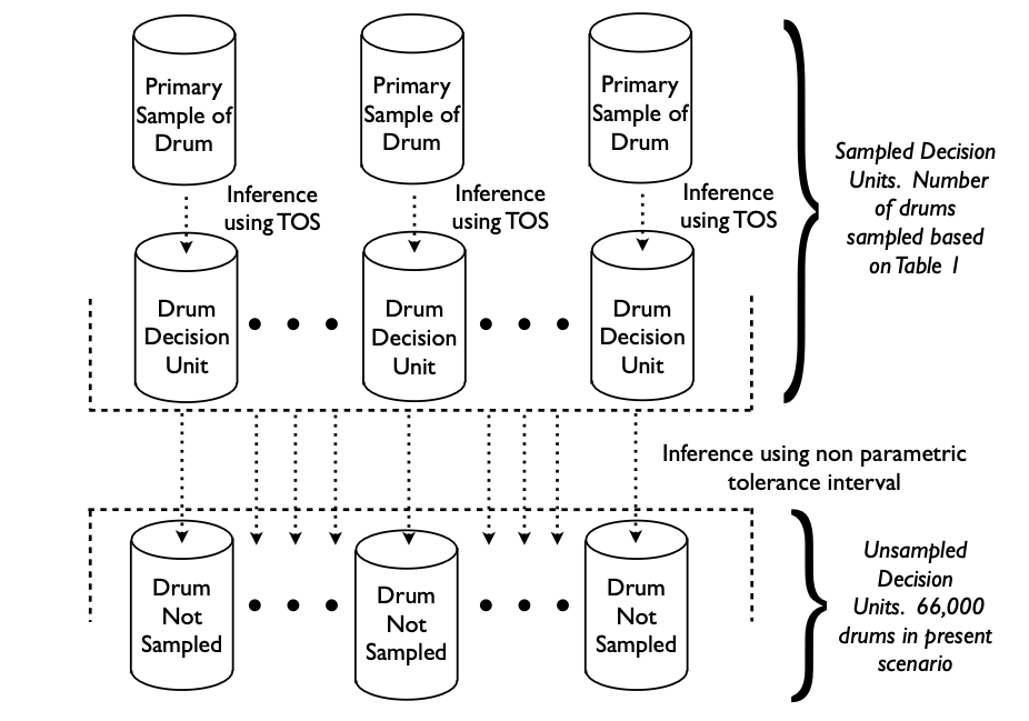
Sampling is nothing more than the practical application of statistics. If statistics were not available, then one would have to sample every portion of an entire population to determine one or more parameters of interest. There are many potential statistical tests that could be employed in sampling, but many statistical tests are useful only if certain assumptions about the population are valid. Prior to any sampling event, the operative Decision Unit (DU) must be established. The Decision Unit is the material object that an analytical result makes inference to. In many cases, there is more than one Decision Unit in a population. A lot is a collection (population) of individual Decision Units that will be treated as a whole (accepted or rejected), depending on the analytical results for individual Decision Units. The application of the Theory of Sampling (TOS) is critical for sampling the material within a Decision Unit. However, knowledge of the analytical concentration of interest within a Decision Unit may not provide information on unsampled Decision Units; especially for a hyper-heterogenous lot where a Decision Unit can be of a completely different characteristic than an adjacent Decision Unit. In cases where every Decision Unit cannot be sampled, application of non-parametric statistics can be used to make inference from sampled Decision Units to Decision Units that are not sampled. The combination of the TOS for sampling of individual Decision Units along with non-parametric statistics offers the best possible inference for situations where there are more Decision Units than can practically be sampled.

Introduction

There are heterogeneous materials and there are heterogeneous lots. Materials can be heterogeneous in the sense of dissimilarity between the fundamental constituent units of the material, e.g. particles (and fragments thereof), grains, minerals, cells biological units … (this is the definition of heterogeneity in the Theory of Sampling, TOS). Lots can be heterogeneous in the sense of dissimilarity between the characteristics of Decision Units (DU). Moreover, there are types of hyper-heterogeneous lots with significant internal complexity, which can be known or hidden. Below, lots of this latter type are in focus.

For many hyper-heterogeneous lots with complex internal structure(s), i.e. lots containing groups of more-or-less distinct DUs, complete sampling is, in practice, often impossible due to logistical, economical or other restrictions. Such lots cannot be sampled reliably on the basis of an assumed distribution, i.e. the distribution of the analyte(s) between the DUs does not follow any known distribution, making the archetype statistical inference based on a known distribution inadequate. Instead, the basis for the statistical inference of these types of lots is the non-parametric one-sided tolerance limit, which can be applied to all types of lots from uniform to hyper-heterogeneous, but which is especially relevant for the type of hyper-heterogeneous lots exemplified in this contribution.

his column shows the critical importance of the application of non-parametric statistical methods when there are more DUs present than can be sampled as an essential complement to the TOS. This situation in fact occurs in very many contexts, for very many sampling targets and materials and lots. What to do?

Different manifestations of heterogeneity

There is heterogeneity, and there is heterogeneity—there are heterogeneous materials within a DU nand there is heterogeneity between DUs. Materials can be heterogeneous in the sense of the TOS reflecting dissimilarity between the constituent units of the material (particles and fragments thereof, grains, cells, other …) within a DU. Readers may be familiar with this type of sampling, see Reference 1 and further key references therein. There is a special focus on heterogeneity in this TOS sense in Reference 2.

Multiple DUs can be heterogeneous in the sense of differences between the characteristics of DUs, which can be defined more-or-less appropriately. An introduction to sampling of lots of this type is found in Reference 3.

Moreover, there are types of heterogeneous lots with even more internal complexity, which may be known or may be hidden. This column presents a rationale for how to sample such hyper-heterogeneous lots, or more precisely how to sample in the presence of heterogeneity both within and between DUs.

A hyper- heterogeneous lot with hidden structure

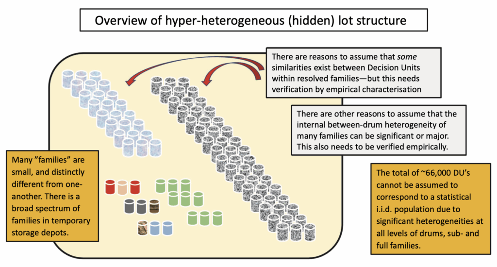
An illustrative example of a hyperheterogeneous lot shall be a legacy nuclear waste mega-lot (see Acknowledgements). Over a period of 50 years, extensive decommissioning of nuclear facilities and several temporary low-level nuclear waste storage facilities have been established, Figure 1, from which waste drums can be retrieved on demand in principle, but in practice associated with various degrees of logistical constraints. In total, there are today ~66,000 conditioned waste drums in temporary storage depots.In 2021–2023 the time has come to start engaging in final end-storage of this legacy nuclear waste. Today there are much stricter Waste Acceptance Criteria (WAC) in play than was the case in earlier decades, for which reason there is a critical need to pre-check “all” drums with the aim of reaching an operative classification into three categories: 1) Cleared for “Final storage”; 2) “Re-classification to intermediate/ high-level storage”; or 3) “Needs further treatment”. The sampling methodology needed for physical, chemical and radiological inspection of selected individual drums has been described by Tuerlinckx and Esbensen.4

The current Herculean task is how to inspect ~66,000 drums for a) physical characteristics; b) chemical characteristics; and c) radioactivity characteristics, which make use of very different types of analytes. With current economic budgets vs the prevailing practical conditions, complete inspection of all ~66,000 drums is likely not feasible, however desirable. In addition, the consequences of an incorrect decision are very serious.

Figure 1. Illustration of a hyper-heterogeneous lot comprised by a hierarchy of units: drums – families – lot. For the discussions
that follow, the operationally relevant DU is an individual drum.

It would have been nice if the ~66,000 drums could be viewed as one statistical population consisting of i.i.d. DUs with a known distribution between DUs (In the nuclear waste realm, often waste drums may even have their own internal heterogeneity, i.e. containing 1, 2 or 3 compressed units (called “pucks”), which may then better reflect the optimal resolved DUs of interest, depending on the specific WAC analytes proscribed. For simplicity in this didactic exposé of statistical methodology however, we here stay with DUs being synonymous with drums.). But because of the 50-year complex decommissioning history it is known that low-level nuclear waste drums not only differ extremely in compositional content(s), physical constitution and radioactivity profiles, but—horror-of-horrors from a statistical point of view—there are very good reasons to infer that there exist groupings within this population of 66,000 DUs. But the degree to which such groupings (“families” in the nuclear expert lingo) are well characterised and well discriminable inter alia, is markedly uncertain; some families are suspected to be clearly demarked, but certainly not all, or maybe not even most.

So far, diligent archival work has resulted in identification of some 40+ “families” or so, each with broadly similar radioactivity profiles. It is relatively easy to measure a radioactive profile fingerprint of an individual drum.4 Due to the marked heterogeneity hierarchy (drums – families – meta-population), Figure 1, it was at one time tentatively decided to try to use “resolved families” as DUs, rather than the entire lot, as laid out by Ramsey.The main statistical issue then was whether it was possible to estimate how many drums would be needed to characterise (or validate) each family with a desired low “statistical uncertainty”. Further comprehensive problem analysis, however, made it clear it was necessary to increase the observation resolution to focus on individual drums as the final operative DUs.

Figure 2. Illustration of inference from multiple sampled to unsampled DUs.

Statistical methodology

The basis for the statistical sampling which must be used for this type of nebulous lot is the non-parametric one-sided tolerance limit, a test that does not depend on any distribution of measurement results. The statistical theory behind this test is described in many statistical text-books. 5–7

Operative statistical approach

Here follows a generic sampling plan that can be applied to hyper-heterogeneous lots in general:

  1. Appropriate definition of DUs in the present scenario, an individual waste drum.
  2. Determine the Data Quality Objectives for the project: Project management must decide its wish for a confidence level (X %) that no more than Y % of the drums may fail the chemical WAC. The confidence level and Y % shall be determined a priori, without any consideration of, or influence from, the statistically required number of samples (see further below). If project management decides to decree 100 % confidence that 0 % fail WAC criteria (a common request), then there is unfortunately nothing that can be done. Then there must be 100 % inspection of all DUs and there must be zero sampling and analytical error – this is obviously an impossibility.
  3. Statistical criterion: Statistical sampling includes the possibility that some failing DUs may be missed. This potential is to be balanced by the tremendous reduction in sampling and analytical costs achievable by carrying out statistical sampling of only a fraction of the total population of DUs. To determine the sampling effort required, the X confidence and Y percent must be determined prior to calculating the required number of drums to be physically sampled. It is the responsibility of project management to decide on its wish independently and a priori of working out the sampling plan. Most importantly, do not first select the required number of samples to be extracted, for example based on project economics, logistics or some other bracketing factor, and then accept what the confidence level and risk percent based on this number turns out to be. The confidence level and risk percent must only be based on considerations of the consequences of an incorrect statistical decision (Table 1).
    Statistical clarification: The percent of drums that may fail does not imply that any of the unsampled drums will fail, just that many could possibly fail and that this would be detectable. The number of samples required for any combination of confidence and proportion of DUs can be determined from the master equation shown in the Appendix illustration, based on Reference 6.
  4. Action plan: Select and retrieve required number of drums at random from the total population of drums. It is imperative that any drum selected in the statistical sampling plan is fully available for sampling and can be extracted without any undue restrictions in practice. Statistical conclusion: If none of the extracted drums fail the chemistry WAC, project management can be “X % confident that no more than Y % of the drums fail the chemical WAC”. Since these Data Quality Objectives have been decided a priori, this means that the project can dispose of all drums in the population without further verification regarding the operative WAC. It is noted that this statistical test assumes that there is no sampling error and no analytical error. While this cannot ever be the case, in practice it is imperative that these errors be controlled as much as possible to provide reliable conclusions, see Reference 8. However—and this is the whopper of all inferential statistics:
  5. If one or more of the DUs fail the chemical WAC criteria, the Data Quality Objectives have not been met, and additional sampling and analysis of drums must be performed. In this case there are several options to continue the characterisation project. It is imperative to develop such alternatives in collaboration with all stakeholders and parties involved, frontline scientific and technical personal, project management, overseeing boards a.o. One possible course of action could be to compare the sampled drums with their radiological profiles to see if there is a correlation between the radiological profile and the chemical parameters in the WAC. There could then, perhaps, be established a multivariate data model, aka a chemometric model.9 If this is the case, it may perhaps be possible to classify all the drums in the population into operative sub-populations (a la the presently resolved ~40 radiological families) as a basis for repeating steps 1–3 above, specifically now addressing the array of resolved sub-populations (“families”) individually. This approach could be attempted for any relevant WAC (radiological, chemical, physical, other …). N.B. This model must be validated on additional random DUs, since it is easy to constrain a model to fit the available data. The critical issue is to test the model, to validate the model on a new set of randomly selected DUs (“test set validation”). The number of samples to verify any model will be that same as initially determined since the data quality objectives do not change. It makes no sense to try out just a moderate number of additional samples. The power of non-parametric statistics lies in the number of DUs with which to cope with hyper-heterogeneous lots; this is a hard problem.
Table 1. Statistically required number of samples to be extracted from a population. In this table, “failing” means a maximum amount that could fail, not implying that any will fail.
The required number of samples can be calculated for any combination of confidence level and percent.
If the number of drums required to be sampled approaches the total number (greater that 10 %) in a population (or in a resolved family or another sub-set of the complex lot), the required number of samples can be reduced by application of the so-called finite population correction. In this case seek further statistical assistance.

Take home lesson

The objective of this issue’s contribution is to present a type of lot heterogeneity for which all types of parametric statistics is not applicable (based on assumed, or proven, normal distribution, nor any other parametric distribution). While the above approach is illustrated by a lot with rather specific features, it well illustrates the general characteristic for which non-parametric statistical inference can deal with complex, partially or wholly, hidden structure(s).

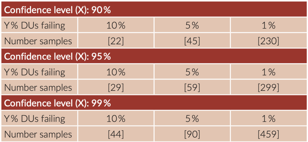
Table 1 shows the evergreen question raised when seeking help from statistics: “how many” observations or measurements are needed in this generic non-parametric approach, presented for a few typical cases i.e. (90, 95, 99 %) confidence that no more than (10, 5, 1 %) DUs could be failing. The smallest vs the largest necessary number of samples needed to allow this test regimen could be from

just a few to thousands, depending on the Data Quality Objectives. The power of generalisation is awesome, since this test scenario is applicable to all kinds of lots (populations) where it is not possible to sample all DUs—that’s quite a broad swath of the material world in which sampling is necessary!

A prominent “someone” from the sampling community, not a professional statistician, when presented with this non-parametric approach for the first time, exclaimed: “But these are magic numbers—they apply to everything, to every lot with such ill-defined characteristics. This is fantastic! Where do these numbers come from?”

The science fiction author Isaac Asimov (Figure 3) once pronounced: “Any sufficiently developed technology, when assessed on the basis of contemporary knowledge, will be indistinguishable from magic”.

Figure 3. Isaac Asimov: he knew a thing or two about science and technology, and the human condition.
Credit: Jim DeLillo/Alamy Stock Photo

 A perspective from the point of view of confidence vs reliability

John Young (1930–2018), by many considered the consummate astronaut, was a.o. the only astronaut to fly both in NASA’s Gemini, Apollo and Space Shuttle programmes; he flew in space six times in all. For an absolutely fascinating life’s story, see Reference 10; or his entry in Wikipedia.

After a “stellar” career as an active astronaut, in 1987 he took up a newly created post at the Johnson Space Center as Special Assistant for Engineering, Operations and Safety. In this position Young became known, rightly so, as the memo guy, producing literally hundreds of memos on all matters related to crew safety, most definitely not afraid to ruffle more than a few feathers when he felt the need. Safety was foremost in his mind. Young knew better than anyone that space flight is a very risky business, but he also knew the importance of paying attention to detail – and always doing things right.

rom this plethora of safety missives, here is a small nugget – a gem rather in the present context (Reference 10, pp. 314–315): “Sometimes the absurdity of bureaucratic logic was tough to take. Consider the case of the solid rocket motor (SRM) igniter. At the flight readiness review for STS-87 (….), we heard a report saying that the solid rocket motor igniter had undergone twelve changes. The changes, along with some other involving the manufacturer, has occasioned the test-firing of six new igniters. Something called “Larson’s Binomial Distribution Nomograph on Reliability and Confidence Levels” indicated that firing six igniters with zero failures gave us 89 % reliability with 50 % confidence. To raise that to 95 % reliability with 50 % confidence would take fourteen firings, while raising it to 95 % reliability with 90 % confidence would take forty-three firings. So, stupid me, I asked that we continue firing igniters to upgrade our confdence. Clearly it was far cheaper, I thought, to gain confidence than to experience a failure of the SRM igniter in what was only a flight test.” Not related to the present column, but interesting, and funny, is Young’s next paragraph: “So, what was the response to my suggestion? I was told that the plant that manufactured the igniters had been moved. Later, I was told that the manufacturing plant had not been moved and, ‘therefore’, firing six igniters should be enough. ‘Therefore?’”

Figure 4. October 1971 portrait photograph of John W. Young. Credit: NASA

Epilogue: carrying over

So, no magic—just the right kind of inferential statistics to the rescue for this type of “difficult to sample” lot or population.

However, an immediate apropos, which is non-negotiable: all physical sampling of the individual DUs selected and extracted, must be compliant with the stipulations, rules and demands for representative sampling laid down by the TOS. This is an essential approach when the destructive testing is required, no exceptions.

There are many other types of lots with similar characteristics as the ones selected for illustration here to be found across a very broad swath of sectors in science, technology, industry, trade and environmental monitoring and control. For example, from the food and feed sector, from which can be found key examples in Reference 11. Or from the mining realm: primary sampling of broken ore accumulations12,13 as brought to the mill in haphazardly collected truck loads, while sampling for environmental monitoring and control is a field in which the present approach finds extensive applications. It is instructive to acknowledge that the within-DU as well as the between-DU heterogeneity characteristics from such dissimilar application fields, food vs ore are identical, it is just a matter of degree.2

Appendix

Where and how to find appropriate “magic numbers”

The Larson nomogram (Figure 5) can be used to obtain the required sample numbers presented in this paper. This nomogram was developed in 1966, long before the proliferation of computers, and is based on the binomial distribution. To use the nomogram, draw a line from the desired “confidence” to the “percent” one is willing to allow to fail. The intersection of that line to the line of “n Sample size” gives the necessary number of samples to inspect. With this methodology, an exact determination is impossible, but readings from the nomogram are consistent with calculated values.

Figure 5. The Larson nomogram. Four circles indicate the required number of samples, found where lines connecting the desired “Confidence” with the desired “Percent” intersect the edge labelled “n Sample size”. Also note bottom part where this edge is labelled “x Number of Defects” (see text). Wikimedia Commons.

Larson developed this nomogram for lot acceptance sampling. Lot acceptance sampling is where and entire lot of individual DUs is accepted or rejected, depending on the acceptable failure rate of individual DUs within the lot. This is very common in statistical quality control. In traditional acceptance sampling any failure rate can be established. In the scenario presented in this paper, the desired failure rate is zero, but that cannot be achieved without 100 % inspection. Therefore, there needs to be balance between the economics of 100 % inspection and the possibility that (a) drum(s) may be mischaracterised.

The Larson nomogram also provides values allowing for some defects—notice that many more samples are required in that case. While it is statistically equivalent, this approach (allowing a few defects) is not applicable for the scenario used in this paper since we here show the case in which we are not willing to knowingly allow any failing DUs. But this possibitity offers an interesting view into even more broad applications, see, for example, References 3, 5, 14–17.

Acknowledgements

The authors acknowledge inspiration to use the generic nuclear waste scenario concept from work with BELGOPROCESS, greatly appreciated. It is clear, however, that the approach described above in this specific context is of much wider general usage ….

References

[] K.H. Esbensen, Introduction to the Theory and Practice of Sampling. IM Publications Open (2020). https://doi.org/10.1255/978-1-906715-29-8

[] K.H. Esbensen, “Materials properties: heterogeneity and appropriate sampling modes”, J. AOAC Int. 98, 269–274 (2015). https://doi.org/10.5740/jaoacint.14-234

[] C.A. Ramsey, “Considerations for inference to decision units”, J. AOAC Int. 98(2), 288–294 (2015). https://doi.org/10.5740/jaoacint.14-292

[] R. Tuerlinckx and K.H. Esbensen, “Radiological characterisation of nuclear waste—the role of representative sampling”, Spectrosc. Europe 33(8), 33–38 (2022). https://doi.org/10.1255/sew.2021.a56

[] R.E. Walpole, R.H. Myers, S.L.Myers and K. Ye, Probability and Statistics for Scientists and Engineers, 9th Edn. Prentice Hall (2011).

[] G.J. Hahn and W.K. Meeker, Statistical Intervals. John Wiley & Sons (1991). https://doi.org/10.1002/9780470316771

[] D.R. Helsel, Nondetects and Data Analysis, Statistics for Censored Environmental Data. John Wiley & Sons (2005).

[] C. Ramsey, “The effect of sampling error on acceptance sampling for food safety”, Proceedings of the 9th World Conference on Sampling and Blending, Beijing (2019).

[] K.H. Esbensen and B. Swarbrick, Multivariate Data Analysis: An Introduction to Multivariate Analysis, Process Analytical Technology and Quality by Design, 6th Edn. CAMO Publishing (2018). ISBN 978-82-691104-0-1

[] J. Young (with James R. Hansen), Forever Young: A Life in Adventure in Air and Space. University Press of Florida (2012). ISBN 978-0-8130-4933-5

[] K.H. Esbensen, C. Paoletti and N. Theix, (Eds), “Special Guest Editor Section (SGE): sampling for food and feed materials”, J. AOAC Int. 98(2), 249–320 (2015).

[] S.C. Dominy, S. Purevgerel and K.H. Esbensen, “Quality and sampling error quantification for gold mineral resource estimation”, Spectrosc. Europe 32(6), 21–27 (2020). https://doi.org/10.1255/sew.2020.a2

[] S.C. Dominy, H.J. Glass, L. O’Connor, C.K. Lam, S. Purevgerel and R.C.A. Minnitt, “Integrating the Theory of Sampling into underground mine grade control strategies”, Minerals 8(6), 232 (2018). https://doi.org/10.3390/ min8060232

[] D. Wait, C. Ramsey and J. Maney, “The measurement process”, in Introduction to Environmental Forensics, 3rd Edn. Academic Press, pp. 65–97 (2015). https://doi.org/10.1016/B978-0-12-404696-2.00004-7

[] C.A. Ramsey and C. Wagner, “Sample quality criteria”, J. AOAC Int. 98(2), 265–268 (2015). https://doi.org/10.5740/jaoacint.14-247

[] C.A. Ramsey and A.D. Hewitt, “A methodology for assessing sample representativeness”, Environ. Forensics 6(1), 71–75 (2005). https://doi.org/10.1080/15275920590913877

[] C.A. Ramsey, “Considerations for sampling contaminants in agricultural soils”, J. AOAC Int. 98(2), 309–315 (2015). https://doi.org/10.5740/jaoacint.14-268

Glossary

A B C D E F G H I J K L M N O P Q R S T U V W X Y Z

A

Aliquot

An aliquot is the ultimate sub-sample extracted in a 'Lot-to-Aliquot' pathway for analysis. By analogy, process analytical technology involves the extraction of virtual samples, which are defined volumes of matter interacting with a process analytical instrument.

Analysis

Analysis is the systematic examination and evaluation of the ultimate sub-sample of chemical, biological, or physical substance (Aliquot) to determine its composition, structure, properties, or presence of specific components.

Analytical Bias

Analytical bias is a systematic deviation of measured values from true values.  An analytical bias can arise from multiple sources, including instrument calibration errors, sample preparation techniques, operator method, or inherent methodological limitations. Unlike random errors, which fluctuate unpredictably, analytical bias consistently skews results in a particular direction. Identifying and correcting this bias is crucial to ensure the accuracy and reliability of analytical data (bias correction).

Analytical Precision

Analytical precision refers to the degree of agreement among repeated analyses of the same aliquot under identical conditions. It reflects the consistency and reproducibility of the results obtained by a given analytical method. High precision indicates minimal random analytical error and close clustering of analytical results around an average. Precision does not necessarily imply accuracy, as a method can be precise yet still yield systematically biased results. 

C

Composite Sampling

Composite sampling extracts a number (Q) of  Increments, established to capture the Lot Heterogeneity. Composite sampling is the only way to represent heterogeneous material. A composite sample is made by aggregating the Q increments subject to the Fundamental Sampling Principle (FSP). The required amount of increments for the requested Representativity Q can be carefully established to make sampling fit-for-purpose.

Compositional Heterogeneity (CH)

Compositional heterogeneity is the variation between individual fundamental units of a target material (particles, fragments, cells, ...). CH is an intrinsic characteristic of the target material to be sampled.

Correct Sampling Errors (CSE)
CSE are the errors that cannot be eliminated even when sampling correctly (unbiased) according to the Theory of Sampling (TOS). CSE are caused by Lot Heterogeneity and can only be minimised.
There are two Correct Sampling Errors (CSE):
  1. Fundamental Sampling Error (FSE)
  2. Grouping and Segregation Error (GSE)
Crushing
Crushing is the term used for the process of reducing particle size. Other terms are grinding, milling, maceration, comminution. Particle size reduction changes the Compositional Heterogeneity (CH) of a material. Composite Sampling and crushing are the only agents with which to reduce the Fundamental Sampling Error (FSE).

D

Data Format

Data must be reported as the measurement results and the Measurement Uncertainties stemming from sampling and analysis. Note that MUAnalysis and MUSampling are expressed as variances.

Data =            Measurement +/- (MUSampling ; MUAnalysis)

Example:       375 ppm +/- (85 ppm ; 18 ppm)

Note that the Uncertainties 85 ppm and 18 ppm are the square roots of MUSampling and MUAnalysis.

Data Uncertainty
Distributional Heterogeneity (DH)

Distributional heterogeneity is the variation between groups of fundamental units of a target material. Groups of units manifest themselves as Increments used in sampling. DH is an expression of the spatial heterogeneity of a material to be sampled (Lot).

DS3077:2024

This standard is a matrix-independent standard for representative sampling, published by the Danish Standards Foundation. This standard sets out a minimum competence basis for reliable planning, performance and assessment of existing or new sampling procedures with respect to representativity. This standard invalidates grab sampling and other incorrect sampling operations, by requiring conformance with a universal set of six Governing Principles and five Sampling Unit Operations. This standard is based on the Theory of Sampling (TOS).

webshop.ds.dk/en/standard/M374267/ds-3077-2024

Dynamic Lot

A dynamic lot is a moving material stream where sampling is carried out at a fixed location. For both Stationary Lots and Dynamic Lots, sampling procedures must be able to represent the entire lot volume guided by the Fundamental Sampling Principle.

F

Fractionation

Fractionation is a way of processing a Lot or Sample before sampling (or subsampling). Fractionation separates materials/lots into fractions according to particle properties, e.g. size, density, shape, magnetic susceptibility, wettability, conductivity, intrinsic, or introduced moisture ...

Fundamental Sampling Error (FSE)

FSE results from the impossibility to fully compensate for inherent Compositional Heterogeneity (CH) when sampling. FSE is always present in all sampling operations but can be reduced by adherence to TOS' principles. Even a fully representative, non-biased sampling process will be unable to materialise two samples with identical composition due to Lot Heterogeneity. FSE can only be reduced by Crushing (followed by Mixing / Blending) i.e. by transforming into a different material system with smaller particle sizes.

Fundamental Sampling Principle (FSP)

The Fundamental Sampling Principle (FSP) stipulates that all potential Lot Increments must have the same probability of being extracted to be aggregated as a Composite Sample. Sampling processes in which certain areas, volumes, parts of a Lot are not physically accessible cannot ensure Representativity.

G

Global Estimation Error (GEE)

The GEE is the total data estimation error, the sum of the Total Sampling Error (TSE) and the Total Analytical Error (TAE).

Governing Principles

Six Governing Principles (GP) describe how to conduct representative sampling of heterogeneous materials:

1) Fundamental Sampling Principle (FSP)

2) Sampling Scale Invariance (SCI)

3) Principle of Sampling Correctness (PSC)

4) Principle of Sampling Simplicity (PSS)

5) Lot Dimensionality Transformation (LDT), and

6) Lot Heterogeneity Characterisation (LHC).

Grab Sampling

Process of extracting a singular portion of the Lot. Grab sampling cannot ensure Representativity for heterogeneous materials. Grab sampling results in a sample designated a Specimen.

Grouping and Segregation Error (GSE)

The GSE originates from the inherent tendency of Lot particles, or fragments hereof, to segregate and/or to group together locally to varying degrees within the full lot volume. This spatial irregularity is called the Distributional Heterogeneity (DH). There will always be segregation and grouping of Lot particles at different scales. GSE plays a significant role in addition to the Fundamental Sampling Error FSE. Unlike FSE however, the effects from GSE can be reduced in a given system state by Composite Sampling and/or Mixing / Blending. GSE can in practice be reduced significantly but is seldomly fully eliminated.

H

Heterogeneity

Heterogeneity refers to the state of being varied in composition. It is often contrasted with homogeneity, which implies complete similarity among components, which is a rare case. For materials in science, technology and industry heterogeneity is the norm. Heterogeneity applies to various contexts, such as populations of non-identical units, bulk materials, powders, slurries, biological swhere multiple distinct components coexist.

Heterogeneity in context of the Theory of Sampling, is described using three distinct characteristics, Compositional Heterogeneity CH, Distributional Heterogeneity DH and Particle-Size Heterogeneity


Heterogeneity Testing (HT)

Heterogeneity tests are used for optimizing sampling protocols for a variable of interest (analyte, feature) with regards to minimising the Fundamental Sampling Error (FSE).

Experimental approaches available are the 50-particle method, the heterogeneity test (HT), the sampling tree experiment (STE) or the duplicate series/sample analysis (DSA), and the segregation free analysis (SFA).

Recently, sensor-based heterogeneity tests have been introduced which bring the advantage of cost-effective analysis of large numbers of single particles.

Homogeneity

An assemblage of material units with identical unit size, composition and  characteristics. There are practically no homogenous materials in the realm of technology, industry and commerce (mineral resources, biology, pharmaceuticals, food, feed, environment, manufacturing and more) of interest for sampling. With respect to sampling, it is advantageous to consider that all materials are in practice  heterogeneous.

I

Incorrect Delimitation Error (IDE)

The principle for extracting correct Increments from processes is to delineate a full planar-parallel slice across the full width and depth of a stream of matter (Dynamic Lot. IDE results from delineating any other volume shape. When a sampling system or procedure is not correct relative to the appropriate Increment delineation, a Sampling Bias will result. The resulting error is defined as the Increment Delimitation Error (IDE). Similar IDE definitions apply to delineation and extraction of increments from Stationary Lots.

Incorrect Extraction Error (IEE)

Increments must not only be correctly delimitated but must also be extracted in full. The error incurred by not extracting all particles and fragments within the delimitated increment is the Increment Extraction Error (IEE). IDE and IEE are very often committed simultaneously because of inferior design, manufacturing, implementation or maintenance of sampling equipment and systems.

Incorrect Preparation Error (IPE)

Adverse sampling bias effects may occur for example during sample transport and storage (e.g. mix-up, damage, spillage), preparation (contamination and/or losses), intentional (fraud, sabotage) or unintentional human error (careless actions; deliberate or ill-informed non-adherence to protocols). All such non-compliances with the criteria for representative sampling and good laboratory practices (GLP) are grouped under the umbrella term IPE. The IPE is part of the bias-generating errors ISE that must always be avoided.

Incorrect Sampling Errors (ISE)

There are four ISE, which result from an inferior sampling process. These ISE can and must be eliminated.

  1. Incorrect Delimitation Error (IDE) aka Increment Delimitation Error
  2. Incorrect Extraction Error (IEE) aka Increment Extraction Error
  3. Incorrect Preparation Error (IPE) aka Increment Preparation Error
  4. Incorrect Weighing Error (IWE) aka Increment Weighing Error
Incorrect Weighing Error (IWE)

IWE reflects specific weighing errors associated with collecting Increments. For process sampling, IWE is incurred when extracted increments are not proportional to the contemporary flow rate (dynamic 1-dimensional lots), at the time or place of extraction. IWE is often a relatively easily dealt with appropriate engineering attention. Increments, and Samples, should preferentially represent a consistent mass (or volume).

Increment

Fundamental unit of sampling, defined by a specific mass or correctly delineated volume extracted by a specified sampling tool.

L

Lot

a) A Lot is made up of a specific target material to be subjected to a specified sampling procedure.

b) A Lot is the totality of the volume for which inferences are going to be made based on the final analytical results (for decision-making). Lot size can range from being extremely large (e.g. an ore body, a ship) to very small (e.g. a blood sample).

c) The term Lot refers both to the material as well as to lot size (volume/mass) and physical characteristics. Lots are distinguished as stationary or dynamic lots. A stationary lot is a non-moving volume of material, a dynamic lot is a material stream (Lot Dimensionality). For both stationary and dynamic lots, sampling procedures must address the entire lot volume guided by the Fundamental Sampling Principle (FSP).

Lot Definition

Lot Definition describes the process of defining the target volume, which will be subjected to Sampling.

Lot Dimensionality

TOS distinguishes Lot volume  according to the dimensions that must be covered by correct Increment extraction. This defines the concept of 'lot dimensionality', an attribute which is independent of the lot scale. Lot dimensionality is a characterisation to help understand and optimise sample extraction from any lot at any sampling stage. There are four main lot types: 0-, 1-, 2- and 3-dimensional lots (0-D, 1-D, 2-D and 3-D lots).

Lots are classified by subtracting the dimensions of the lot that are fully 'covered' be the salient sampling extraction tool in question. The higher the number of dimensions fully covered in the resulting sampling operation, the easier it is to reduce the Total Sampling Error TSE.

Lot Dimensionality Transformation (LDT)

By the Governing Principle Lot Dimensionality Transformation LDT, stationary 0-D, 2-D and 3-D lots can in many cases advantageously be transformed into dynamic 1-D lots, enabling optimal sampling. However, the application of LDT has practical limits as some lots cannot be transformed (e.g. a body of soil, or a mine resource, biological cells). The optimal approach for such cases is penetrating one dimension with complete increment extraction (usually height) turning a 3-D lot into a 2-D lot.

Lot Heterogeneity

The lot heterogeneity is the combination of Compositional Heterogeneity, Distributional Heterogeneity and Particle-Size-Heterogeneity.

CH + DH + PH

Lot Heterogeneity Characterisation
Lot Heterogeneity Characterisation is the process of assessing Lot Heterogeneity magnitude. Logically, it is impossible to design a sampling procedure without knowledge of the Heterogeneity of target material. Lot Heterogeneity Characterisation is the process of determining Lot Heterogeneity when approaching a new sampling project. There are two principal procedures of determining Lot Heterogeneity, Replication Experiment (RE) for Stationary Lots, and Variographic Characterisation (VAR) for Dynamic Lots. Heterogeneity Tests determine Constitutional Heterogeneity as the irreducible minimum obtainable of Sampling Variance, excluding all other Sampling Error effects.

M

Mass-Reduction

Mass-reduction is a physical process that divides a given quantity into manageable sub-samples. Mass-reduction must ensure that these sub-samples are representative of the original quantity (Representative Mass Reduction – Subsampling

Measurement

The total process of producing numerical data about a Lot, including sampling and analysis is called Measurement. Simultaneously, sensor-based analytical technology combines virtual sampling and signal processing. For both types of measurements the principles and rules of the  Theory of Sampling apply.

Measurement Uncertainty (metrological term) (MU)

MU expresses the variability interval of values attributed to a quantity measured. MU is the effect of a particular error, e.g. a sampling error, or an analytical error  or of combined effects (see MUTotal).

MUsampling reflects the variability stemming from sampling errors

MUanalysis reflects the variability stemming from analytical errors

MUtotal is the effective variability stemming from both sampling and analysis

MUtotal= MUsampling+ MUanalysis

Mixing / Blending

Mixing and blending reduces Distributional Heterogeneity (DH) before sampling/sub-sampling. N.B. Forceful mixing is a much less effective process than commonly assumed.

P

Particle-Size-Heterogeneity (PH)

PH is the compositional difference due to assemblages of units with different particle sizes (or particle-size classes).

Pierre Gy

The founder of the Theory of Sampling (TOS), Pierre Gy (1924--2015) single-handedly developed the TOS from 1950 to 1975 and spent the following 25 years applying it in key industrial sectors (mining, minerals, cement and metals processing). In the course of his career he wrote nine books and gave more than 250 international lectures on all subjects of sampling. In addition to developing TOS, he also carried out a significant amount of practical R&D. But he never worked at a university; he was an independent researcher and a consultant for nearly his entire career - a remarkable scientific life and achievement.

Precision

Precision is a measure of the variability of quantitative results. The larger the variability, the smaller the precision. In practice, precision is measured as the statistical variance s2 of the quantitative results (square of the standard deviation).

Primary Sample

The initial mass extracted from the lot. The Primary Sample is the product of Composite Sampling and consists of Q Increments. Both the mass of the Primary Sample as well as the number of increments extracted influence the sampling variability. As the primary sampling stage often has by far the largest impact on MUTotal, optimisation always starts at this stage.

Principle of Sampling Correctness (PSC)

The Principle of Sampling Correctness (PSC) states that all TOS' Incorrect Sampling Errors (ISE) shall be eliminated, or a detrimental Sampling Bias will have been introduced.

Principle of Sampling Simplicity (PSS)

PSS states that sampling along the Lot-to-Aliquot can be optimised separately for each (primary, secondary, tertiary ....) sampling stage. Since the Primary Sampling stage is often the dominant source of sampling error, optimization logically shall always begin at this stage.

Process Periodicity Error (PPE)

PPE is incurred if short-, mid- or long-term periodic process behaviour is not corrected for, in which case it may contribute to a sampling bias.

A process sampling strategy must make use of a high enough sampling frequency to uncover such behaviours; the sampling frequency must as a minimum always be higher than twice the most frequent periodicity encountered.

Process Sampling Errors (PSE)

PSE come into effect when Dynamic Lots are being sampled without compensating for process trends or periodicities (Process Trend Error and Process Periodicity Error).

Process Trend Error (PTE)

PTE occurs if mid- to long-term process trends are not corrected for, in which case they may contribute to a Sampling Bias. PTE and Process Periodicity Error PPE may, or may not, occur simultaneously depending on the specific nature of the process to be sampled.

Q

Q

Number of Increments composited to a Sample.

R

R

R is the number of replications of a series of independent complete ‘Lot-to-AliquotMeasurements, made under identical conditions applied in a Replication Experiment.

Replication Experiment (RE)

The replication experiment RE consists of a series of independent complete ‘Lot-to-Aliquot’ analytical determinations, made under identical conditions. The number of replications is termed R. RE provides MUSampling + MUAnalysis.

Representative Mass Reduction – Subsampling

Representative Mass Reduction (RMR) aka sub-sampling. TOS argues why Riffle-Splitting and Vezin-sampling are the only options leading to Representative Mass Reduction.

Representativity

A sampling process is representative if it captures all intrinsic material features, e.g., composition, particle size distribution, physical properties (e.g. intrinsic moisture) of a Lot.Representativity is a characteristic of a sampling process in which the Total Sampling Error and Total Analytical Error have been reduced below a predefined threshold level, the acceptable Total Measurement Uncertainty.
Representativity is the prime objective of all sampling processes. The representativity status of an individual sample cannot be ascertained in isolation, if removed from the context of its full sampling-and-analysis pathway. The characteristic Representative can only be accorded a sampling process that complies with all demands specified by TOS (DS3077:2024).

S

Sample

Extracted portion of a Lot that can be documented to be a result of a representative sampling procedure (non-representatively extracted portions of a Lot are termed Specimens).

Sampling

Sampling is the process of collecting units from a Lot (sampling procedure; sampling process): Grab Sampling or Composite SamplingThere are only two principal types of sampling procedures: Grab Sampling or Composite Sampling.

Sampling Accuracy

Closeness of the analytical result of an Aliquot with regards to the true concentration of the Lot]/glossary]. NB. “sampling accuracy” = “sampling + analytical accuracy”

Sampling Bias

The Sampling Bias is the difference between the true Lot concentration and the average concentration from replicated sampling. Such a difference is a direct function of the Lot Heterogeneity and as such inconstant; it changes with each additional sampling and can therefore not be corrected for. This is the opposite to the Analytical Bias for which correction is often carried out.

Sampling Error Management (SEM)

SEM determines the priorities and tools for all sampling procedures in the following order:

  1. Elimination of Incorrect Sampling Errors (ISE) (unbiased sampling)
  2. Minimisation of the remaining Correct Sampling Errors (CSE)
  3. Estimation and use of s2(FSE) is only meaningful after complete elimination of ISE
  4. Minimisation of Process Sampling Errors
Sampling Manager

The Sampling Manager is the Legal Person accountable for ensuring that all sampling activities are conducted in accordance with scientifically valid principles to achieve representative results. They are responsible for managing the design, implementation, and evaluation of sampling protocols while balancing constraints such as material variability, logistics, and resource limitations. This role requires expertise in the Theory of Sampling (TOS), leadership, project management and stakeholder communication skills.

Sampling Precision

The Sampling Precision is the variance of the series of analytical determinations, for example from a Replication Experiment (RE). Sampling precision always includes the Analytical Precision, since all analysis is always based on an analytical Aliquot, which is the result of a complete 'Lot-to-Aliquot' sampling pathway. Therefore sampling precision = sampling + analysis precision.

Sampling Protocol

Document explaining the undertakings necessary for the sampling process. It contains the tools and procedures from Lot-to-Aliquot[/glossary].

Sampling Scale Invariance (SCI)

The Principle of SSI states that all Sampling Unit Operations (SUO) can be applied identically to all sampling stages, only the scale of sampling tools differs.

Sampling Uncertainty

Sampling Uncertainty is the difficulty of collecting a representative sample due to Lot Heterogeneity; the more heterogeneous the material, the higher the uncertainty associated with any sample attempting to represent the whole Lot.

Sampling Unit Operations (SUO)
A Sampling Unit Operation is a basic step in the 'Lot-to-Aliquot' pathway. Five practical SUOs cover all necessary practical aspects of representative sampling: Composite Sampling, Crushing, Mixing/ Blending, Fractionation, and Representative Mass Reduction - Subsampling.
Secondary Sample

A secondary sample is the product of Representative Mass Reduction - Subsampling from a Primary Sample. Identical nomenclature applies for further Representative Mass Reduction steps (Tertiary...).

Specimen

A specimen is a portion of a larger mass/volume (Lot) extracted by a non-representative sampling process. Grab Sampling results in a specimen.

Stakeholder

A Stakeholder is any entity interested in the result coming from sampling and analysis. Data representing stationary or flowing heterogeneous materials are requested by different parties with a multitude of differing objectives. Stakeholders can be internal, from commercial organisations, public authorities, research and academia or non-governmental organisations.

Stationary Lot

A Stationary Lot is a non-moving volume of material where sampling is carried at from multiple locations, each resulting in an Increment. For both Stationary Lots and Dynamic Lots, sampling procedures must address the entire Lot volume guided by the Fundamental Sampling Principle (FSP).

T

Theory of Sampling (TOS)

TOS Theory and Practice of Sampling: necessary-and-sufficient framework of Governing Principles (GP), Sampling Unit Operations (SUO), Sampling Error Management rules (SEM) together with normative practices and skills needed to ensure representative sampling procedures. TOS is codified in the universal standard DS3077:2024.

Total Analytical Error

TAE is manifested as the Measurement Uncertainty resulting only from analysis (MUAnalysis). TAE includes all errors occurring during assaying and analysis (e.g. related to matrix effects, analytical instrument uncertainty, maintenance, calibration, other), as well as human error.

Total Measurement Uncertainty

Whereas Measurement Uncertainty (MU) is traditionally only addressing analytical determination, e.g. concentration := 375 ppm +/- 18 ppm (MUanalysis), Theory of Sampling (TOS) stipulates reporting analytical results with uncertainty estimates from both sampling and analysis.  This gives users of analytical data the possibility to evaluate the relative magnitudes of MUsampling vs. MUanalysis, enabling fully informed assessment of the true, effective data quality involved. A complete data uncertainty must have this format:

MUTotal = MUSampling + MUAnalysis

The attribute Total Measurement Uncertainty (MUTotal) is the most important factor determining the attribute data quality.

Total Sampling Error (TSE)

The Incorrect Sampling Errors (ISE) and Correct Sampling Errors (CSE) add up to the effective Total Sampling Error (TSE). TSE is causing the Total Uncertainty resulting from material extraction along the sampling pathway from-lot-to-aliquot (MUSampling).

Total Uncertainty Threshold

The acceptable Total Measurement Uncertainty, which must include the Sampling Measurement Uncertainty (MUSampling) and Analytical Measurement Uncertainty (MUAnalysis).

U

V

Variographic Characterisation (VAR)

Variography is a variability characterisation of a dynamic 1-dimensional dynamic lot. A variogram describes variability as a function of Increment pair spacing (in time). Variography is also applied in geostatisctics in describing the variability as a function of spacing/distance between analyses.