Danish geology icon Arne Noe-Nygaard picks up on an 800 years old sampling and invents the Replication Experiment: PAT in disguise

Kim H. Esbensen1

1 Independent researcher, professor, owner KHE Consulting, Copenhagen, Denmark. www.kheconsult.com

This column showcases the extraordinarily versatile Replication Experiment (RE). Although presented and illustrated before within the professional sampling community, there are still many cases showing inspiring, didactic applications allowing a broader view on the types of “analysis” associated with sampling. Although so-called “economic geological processes” are of key importance within the traditional field(s) of sampling (TOS), i.e. mineralisations, ore exploration and mining, minerals processing, the column author and editor, here drags the reader into a realm very rarely visited in the sampling realm—academic geology. The present case could just as well have been termed “Danish medieval churches meet inspiring geologic icon inventing the RE independently of the TOS”.

Arne Noe-Nygaard, Danish geologist (1908‒1991)

Noe-Nygaard was a Nestor in Danish and Scandinavian geology through a long and very productive academic career. He was a professor for 40 years, also widely involved in popularising geology and was intimately involved in the founding of The Geological Survey of Greenland (GGU, now GEUS). His biography in Wikipedia is unfortunately only in Danish, but visit it anyway—lots of geology is communicated in pictures, images and maps, and his extensive oeuvre is liberally written in English and German, scientifically spanning from the Pre-Cambrium era in Greenland and Denmark to the present (the Quaternary) with a focus on volcanology in Iceland, Greenland and the Faroe Islands, as well as many other topics, one of which is presented in the present column.

A most unusual sampling setting

The present exposé is based on what turned out to be Noe-Nygaard’s last book publicat ion, titled Larvikitter i Kvaderstenskirke (DGU Publ. 1991) ISBN 87-88640-74-4 [Larvikites in hewn stone churches].1

Figure 2. Front page of Larvikites in Hewn Stone Churches published posthumously in 1991. Arne Noe-Nygaard died on 4 June 1991, but managed to edit the first proof of the book just before passing. An active geologist and scientist right up until the end.

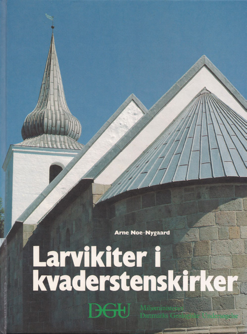
Barely of book size (only 32 pages), it tells a fascinating geological detective story about the provenance of wall rocks in Danish medieval stone churches in northern and western Jutland. As the name implies, this type of church is built by square hewn rocks of local origin from the local landscape in medieval times. But their ultimate origin is much older—and this is the red line of this column.

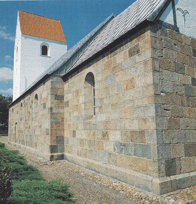
The Romanesque hewn rock churches in Jutland were constructed in the period 1100‒1200. There are still some 700 of them in a reasonably wellpreserved state. In fact, this type of church is rather unique for the northern and western parts of Jutland, hardly found anywhere else in the world.1,2 It is the professional historical view that the source for the rocks used for the original church building is local, i.e. they represent the surrounding landscape from where they were transported as short distances as possible before being hewn, probably at the church site. It is easy to compensate for later alterations and additions regarding improvements and modifications often with a distinct later architectural style, e.g. as seen in Figures 2 and 3 (enlargement of windows, lead roofing and addition of a bell tower). Compensating for this, the geologist Noe-Nygaard shared the belief that most of the original church walls in northern and western Jutland represent a wellpreserved sample of the local rocks found on the surface at the time of building.

Figure 3. “Asp Kirke”, Jutland, typical medieval Romanesque church illustrating the diverse assembly of hewn rock types. Note later improvement (enlargement) of windows, later lead roofing and addition of a bell tower.

But why, and how did the medieval landscape come to be strewn with an abundance of boulders and rocks of a size that would suffice well for production of hewn rocks? This is where an underlying relationship between geology and religion has its origin. It is a fascinating story that involves “erratics”…

Erratics—composition, origin, glacial transportation

Of the use in everyday language (Meriam‒Webster) has the following to say: “Erratic can refer to literal ‘wandering’. A missile that loses its erratic path, and a river with lots of twists and bends is said to have an erratic course. Erratic can also mean ‘inconsistent’ or ‘irregular’. So, a stock market that often changes direction is said to be acting erratically; an erratic heartbeat can be cause for concern; and if your car idles erratically, it may mean that something’s wrong with the sparkplug wiring”.

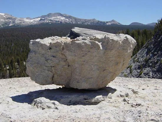
In geology, however, this term is distinctly specific. Here erratic is used in one particular sense only, regarding composition, provenance and direction and distance travelled. Glacial erratics are stones and rocks that were transported by a glacier and were left behind after the glacier melted and retreated. Thus, glacial erratics were formed by erosion (“plucking”) as a result from the flowing movement of ice over the local bedrock. Such erratics can range in size from pebbles to large boulders and can have been carried for hundreds of kilometres (800 km is an often quoted maximum). Scientists have a.o. used erratics to help determine ancient glacier movement(s), i.e. directions, distances and other local features. Particularly large erratics end up as marked landscape elements, Figure 4, sometimes associated with much later local historical lore.

Figure 4. Archetypal “erratic”. The composition of the conspicuous rock may be similar to the local rock types (short distance travelled only) but, much more often, is of markedly different habitus [travelled over long(er) distances]. CredIt: Daniel Mayer, Creative Commons Attribution- Share Alike 1.0 Generic, Encyclopædia Britannica

Of specific interest to the uninitiated reader, and directly related to the story in this column, is the fact that erratics differ in composition and hence in appearance from the local bedrock upon which they are found; of course, mostly clear to the trained geologic eye. Erratics may be embedded in the finegrained, ground up glacial deposits (called till), or, more often, occur as conspicuously independent “special” landscape elements on the bare ground surface.

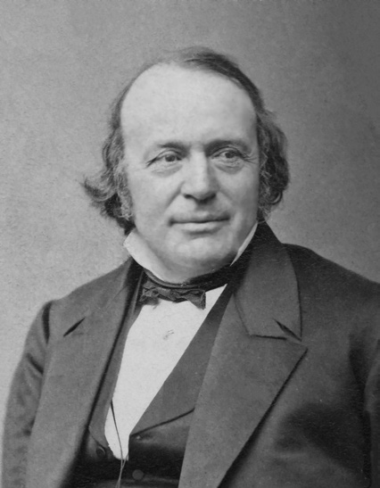
Those transported over long distances generally consist of rock resistant to the shattering and grinding effects of glacial transport. Erratics composed of unusual and distinctive rock types can, by diligent and competent geologists, sometimes be traced to their source of origin and thereby serve as indicators of the direction of glacial movements. Studies making use of such indicator erratics have provided information on the flow paths of the major ice sheets in the ice age(s) of our planet (and indeed also on occasion the location of important mineral deposits). Erratics played an important part in the initial recognition of the most recent ice age(s) and their extent. Originally thought to be transported by gigantic floods or by ice rafting, erratics were first correctly explained in terms of glacial transport by the Swiss‒ American naturalist and geologist J.L.R. Agassiz in 1840.

Figure 5. J.L.R. Agassiz (1840). Photo: Wikipedia, Public Domain

For more information, see the comprehensive entry on glacial erratics in Wikipedia: https:// en.wikipedia.org/wiki/Glacial_ erratic. In this widely covering entry on glacier-borne erratics, a wealth of examples are described, from Australia, Canada, Estonia, Finland, Germany, Republic of Ireland, Latvia, Lithuania, Poland the United Kingdom and the USA. Curiously, however, there is a distinct lacuna: Norway and Denmark are completely missing, which is a major affront to geologists from these two countries, something to be rectified with a friendly vengeance below!

Zooming in…

The reader is now in possession of the necessary subject-matter background for the denouement of this column. Here are the telling detective clues:

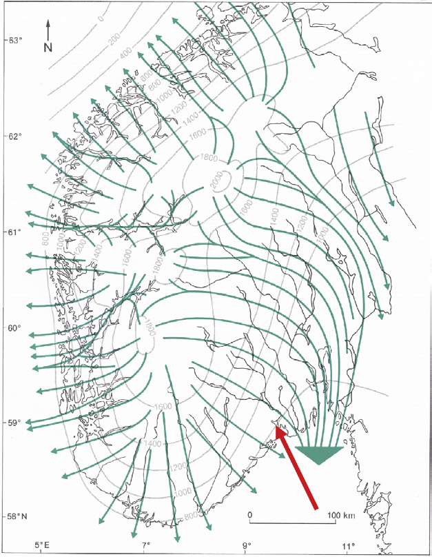
1) Larvikite is a distinct igneous rock formed by solidifying magma, not as a lava, but as a deep-seated intrusive magmatic body in the Earth’s crust. Figure 8 below also shows the source area of known larvikite occurrences in Norway. Igneous rock types are named after the location of the occurrence of the type rock where and when it was first described scientifically.

A few facts of interest:

1) Larvik (https://en.wikipedia.org/wiki/Larvik) is the birth town of the world renowned Norwegian explorer and historian Thor Heyerdal of Kontiki expedition fame.

2) The author of the present column also resided in Larvik for an extended period of time (1980‒2000), from which grew a fascination with the particular rock type in question here. The city itself is immensely proud of its world renowned resources of dimension stone, in the form of polished façade rocks, a major export asset.

3) For a thorough description of the geology of larvikite, the comprehensive publication by Heldal et al. (2008) which, although written for professionals, can also be browsed with pleasure by interested parties: https:// www.ngu.no/upload/Publikasjoner/Special%20publication/SP11_02_ Heldal.pdf

2) There are no occurrence of bedrocks of the larvikite type in Denmark—none!

3) But, very many hewn rock churches in the northern and western-most parts of the Jutland peninsula of Denmark contain a definite, identifiable proportion of larvikite rocks in their makeup. There are actually seven recognisable sub-types (varieties) of larvikite involved, which is for the professional geologists to keep track of, but no worries: Noe-Nygaard knew his larvikites!

4) So how come there were decidedly non-native, indeed “erratic” rock types to be found in the walls of medieval churches in Jutland? This was a major mystery at the time when the science of geology was developing in the 19th century. For example, it was suggested that major floods could have been responsible for such marked dislocations, but after the Agassiz breakthrough (1840), a modern understanding was quickly worked out: in earlier times large(r) parts of the continents in the northern hemisphere were covered (one, or several times) by thick sheets of ice, glaciers (really thick ice sheets, e.g. up to 3 km as in the present day inland ice sheet covering Greenland). Erratics were now envisaged as having been transported by the internal flow of ice masses during a specific (or possible recurrent) glacier event(s) during a specific ice age. An important part of this development is concerned with the evidence and the relics left by scouring ice flows interacting with the bedrocks over which it flows, plucking, plucking …). There is an absolutely overpowering force at work at the bottom of thick ice flows.

5) So, it is no longer a mystery that, for example, larvikite erratics can now be found in Denmark several hundreds of km south of their point of origin; this picture is today well known and accepted. But the details of filling out this broad framework still leaves a lot of complex and highly fascinating questions, answers to which have been worked out by later generations of geologists, and this is where the legacy of Arne Noe-Nygaard’s last book comes to the fore. Questions like from which of the three major ice ages that can be recognised in Denmark did this erratic complement of surfacefound stones originate? (There are several other, intricate details involved here, which find their resolution at the end of Noe-Nygaard’s account, but these can safely be left to the professional connoisseurs of Quaternary glacial geology). Here we leave such particulars and move fast forward to sampling and analysis in this fascinating context.

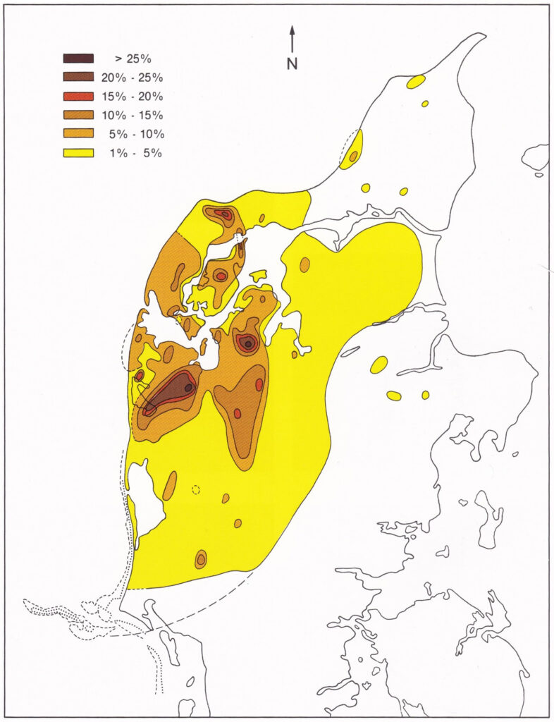
6) Noe-Nygaard’s book gives readers a highly personal tour de Jylland in the form of numerical accounts of the assemblages of hewn rocks to be found in the makeup of the walls of the gamut of Roman churches, broadly constructed in the period 1100‒1200. The final result of Noe-Nygaard’s investigation is reproduced below as Figure 7, to be further commented upon.

In medias res: sampling and analysis

So, what kind of sampling was used in this story? And what kind of analysis?

One could perhaps imagine that church wall rocks were sampled in the traditional field geological sense with “field samples” brought to the laboratory for petrological, mineralogical and geochemical analysis with a view of identifying the different type of larvikite rocks and thus their proportions of the complete hewn rock church assembly. But no, the story is more interesting, and far more personal in a unique sense. In today’s sampling and analysis terms as used in science, technology and industry, Noe-Nygaard unknowingly made use of what today is known as a “PAT-approach”, although the concept of Process Analytical Technology was not to be established until years later than Noe-Nygaard’s first field investigations.

A PAT aside

The key aspect of PAT is to perform sampling and analysis in one-andthe- same-operation. Within PAT the focus is nearly always on the many contending analytical modalities competing for attention and each claiming superiority, but there is also an underlying, unfortunately often unrecognised challenge, related to the role of the sampling interface.

The key characteristic of PAT is deployment of sensor technologies (physical probes, chemical sensors, other sensors) intercepting and interacting with a process stream. The key characteristic of PAT is that of performing sampling and analysis simultaneously as one unified process: probes and sensors interact analytically with an often small (sometimes minute) “effective volume” of the flux of matter which represents the support volume from which analytical signals are acquired. This is very often in the form of multi-channel spectroscopic signals, which can be transformed into a predicted chemical or physical measurement, see, for example, the fundamental textbook by Katherine Bakeev, Process Analytical Technology,3 in which chemometrics has made essential contributions by deploying the powerful multivariate calibration approach, e.g. Esbensen & Swarbrick.4

Methods and equipment of process sampling are front and centre in the realm of the Theory of Sampling (TOS). The TOS supplies a comprehensive, well-proven framework that derives all principles and implementation demands needed for how to extract representative physical samples from moving lots, i.e. from a conveyor belt or from ducted material streams. PAT aspires to take this situation over to the situation in which the task is how to extract representative sensor signals instead of physical samples.

For “sensor sampling”, i.e. PAT, there is no similar foundational framework. Instead, a pronounced practical approach is evident in this realm, in which the question of how to achieve representative sensor signals is not so much related to the design and implementation of an appropriate sampling interface between the sensor and the streaming flux of matter. Rather, a survey of the gamut of sensor interfaces presented in industry and in the literature reveals a credo that appears to be: “Get good quality multivariate spectral data—and chemometrics will do the rest”, exclusively relying on multivariate calibration of process sensor signals (multi-channel analytical instruments). There is a tacit misunderstanding that the admittedly powerful chemometric data modelling is able to take on and correct for any kind of sensor signal uncertainty—including “sampling errors”. However, this leaves analytical representativity the victim of imperfect under signals, which can be transformed into a predicted chemical or physical measurement, see, for example, the fundamental textbook by Katherine Bakeev, Process Analytical Technology,3 in which chemometrics has made essential contributions by deploying the powerful multivariate calibration approach, e.g. Esbensen & Swarbrick.4 Methods and equipment of process sampling are front and centre in the realm of the Theory of Sampling (TOS). The TOS supplies a comprehensive, well-proven framework that derives all principles and implementation demands needed for how to extract representative physical samples from moving lots, i.e. from a conveyor belt or from ducted material streams. PAT aspires to take this situation over to the situation in which the task is how to extract representative sensor signals instead of physical samples. For “sensor sampling”, i.e. PAT, there is no similar foundational framework. Instead, a pronounced practical approach is evident in this realm, in which the question of how to achieve representative sensor signals is not so much related to the design and implementation of an appropriate sampling interface between the sensor and the streaming flux of matter. Rather, a survey of the gamut of sensor interfaces presented in industry and in the literature reveals a credo that appears to be: “Get good quality multivariate spectral data—and chemometrics will do the rest”, exclusively relying on multivariate calibration of process sensor signals (multi-channel analytical instruments). There is a tacit misunderstanding that the admittedly powerful chemometric data modelling is able to take on and correct for any kind of sensor signal uncertainty—including “sampling errors”. However, this leaves analytical representativity the victim of imperfect understanding of the nature of data analytical errors (ε) vs sampling errors (TOS errors).

In the current PAT focus, representativity is wholly related to spectral and reference sample measurement uncertainty (MU) and to possible data modelling errors, which unfortunately ignores the geometric specifics of sensor signal acquisition in relation to the full cross-section of the streaming/ ducted flux of matter even though this is the very domain where sampling errors occur in the exact same fashion as when extracting physical samples. The process sampling interface comes to the fore.

And this PAT framework relates to the rock assemblages in medieval Danish churches 800 years old—how?

Unknowingly, Arne Noe-Nygaard devised a quite similar simultaneous sampling and analysis approach, in his case in the form of field sampling and analysis all in one. But interesting, his field sampling was not the traditional geological sample collection for analysis in the laboratory.

Field rock identification: field sampling and analysis in one!

So here is how Noe-Nygaard went about his analysis, i.e. visual rock type identification (aka “rock classification”), based on decades of experience with this kind of rock in Scandinavia. Noe-Nygaard was a very experienced geologist able to recognise all the seven major kinds of syenitic rocks making up the family of larvikites.

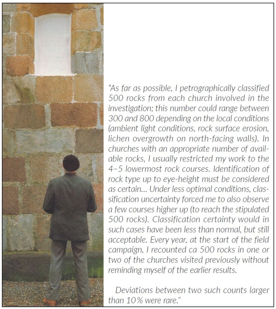
And now the story gets historical. The field sampling part (gathering the local surface rocks from the landscapes in Jutland) was undertaken by the original medieval church builders, who, with absolute certainty, were inspired and driven by very different motivations than science—masonry has it origin in the religious wish to build churches in which to worship. It was Arne Noe-Nygaard’s inspired geological brilliance to make explicit this hidden sampling aspect of medieval church building.1,2 Sampling by religious proxy! Thus, each medieval church takes on the role as a (rather large) sample of local landscape boulders, the size of which amounts to the cumulative wall area of the lowermost 5‒7(8) rock courses. In passing (a treat for TOS experts), one observes that samples of this type are comprised by very, very large “particles”, making it imperative to be able to obtain a large enough square footage—the stated minimum of ca 500 rocks (see magazine front cover for a deliberate pointed focus).

Then, with a delay of some 800 years, fast forward to “analysis”— field rock identification, Figure 6.

Figure 6. Geological maestro Arne Noe-Nygaard in the field, at work identifying (and counting) hewn rock types in a population of Romanesque medieval churches in Jutland.

From this field geological rock identification, the proportions of each larvikite rock (and, therefore, also their cumulative count) could easily be calculated as relative % w.r.t. all rocks counted for each church, which results were then plotted on a geographical map of Jutland, Figure 7.

Figure 7. Relative % occurrence of larvikites (sum of all identifiable types) in Jutland hewn rock churches. The field work for this remarkable compilation was undertaken in a series of intermittent summer campaigns by Noe-Nygaard during his tenure as professor at University of Copenhagen, see Noe-Nygaard.1,2

To close the geological part of the story, Figure 8 shows the most recent ice age glacial flow direction patterns in southern Norway. For the reader not familiar with the geography and Quaternary geology of Scandinavia, Denmark is situated some 200 km south of the Norwegian glacial flow field shown. Herewith the connection between identifiable, diagnostic erratics from the area surrounding Larvik in southern Norway and medieval church rock assemblages in Jutland, Denmark, should be fully established and understandable for all, no specialised geological competence needed.

Figure 8. Ice age glacial flow direction patterns in southern Norway, see Nesje et al. (1988).5 Contours show the modelled surface of the glacier in late-Weichsel (ca 20,00 years ago). Illustration with permission from GEUS.

The TOS point: the RE

The point to this extensive geological introduction is the key theme of this sampling column, novel applications of the RE.

Noe-Nygaard was acutely aware that there was an inherent “analytical error” involved in his visual identifications (TAE in today’s parlance of the TOS). Such was his awareness of his analytical performance that he devised his own RE. A translation (KHE) from the Danish in Noe-Nygaard (1991) is presented in Figure 6.

This is it! What a wonderful example of a conscientious scientist, aware that his professional classification performance (analytical performance) is associated with a significant non-zero uncertainty that must be considered. What is remarkable here is that, for geologists, the ability to identify rock types (and mineral species) is a matter of intense professional pride—this is what distinguishes a competent field geologist. One does not question a geologist’s rock identification competence!

And yet, in spite of his very impressive academic a.o. achievements, Arne Noe-Nygaard’s example of professional self-awareness is a remarkable, humble reminder to all scientists, technologists and samplers of today!

Figure 9. “So how difficult can it be?” if one believes one is familiar with syenites from southern Norway, that is. The author of this column could not resist this temptation when driving past an especially inviting hewn rock church during a summer holiday in 2019. Not surprisingly, it turned out to be quite a challenge to even try to best the master geologist Noe-Nygaard, RE < 10 %.

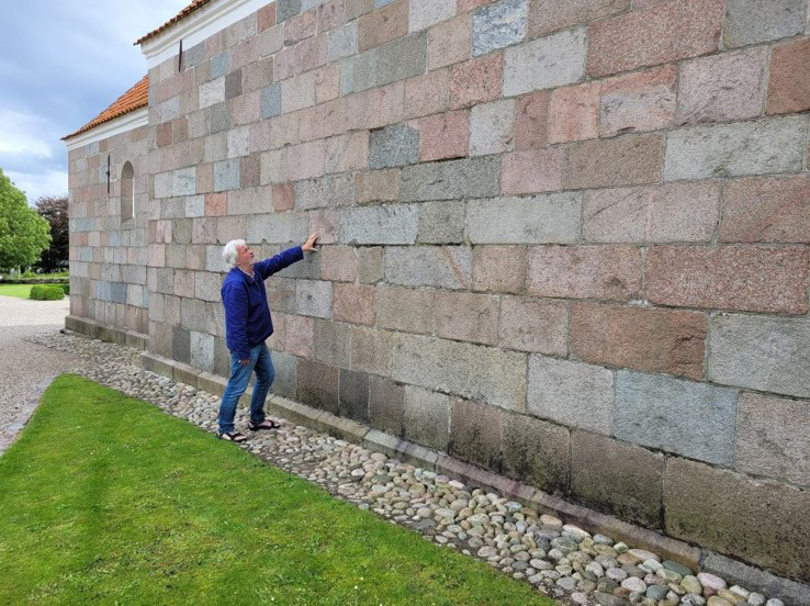
But it is never an easy matter following the footsteps of a giant, Figure 9, not even for a geologist familiar with igneous rocks and who has lived 10 years in Larvik! A first foray comparison of performance uncertainty (RE%), performed during a summer 2019 vacation tour in Jutland taking in a number of beautiful medieval country churches, revealed just how good Arne Noe-Nygaard was to his metier. To be honest, and to Noe-Nygaard’s legacy, his “<10 %” RE uncertainty vastly outshined the score for the hopeful contemporary geologist in Figure 9 (IF the reader must ask, the answer is “a considerable larger percentage”).

Conclusion

The RE is a very versatile facility for evaluating the total uncertainty [TSE + TAE] of any measurement system in which sampling plays a role. While RE has a plethora of manifestations within traditional sectors in technology, industry, commerce, trading and society, this column treated an unusual application of RE thinking hidden away Figure 9. “So how difficult can it be?” if one believes one is familiar with syenites from southern Norway, that is. The author of this column could not resist this temptation when driving past an especially inviting hewn rock church during a summer holiday in 2019. Not surprisingly, it turned out to be quite a challenge to even try to best the master geologist Noe-Nygaard, RE < 10 %. in a most unsuspected niche in academic geology. A famed Danish geologist devised his very own PAT-like sampling-analysis confluence spanning no less than 800 years. What’s not to like?

References

[1] A. Noe-Nygaard, Larvikiter I Kvaderstenskirker. Danmarks Geologiske Undersøgelse, Miljøministeriet, Editor Stig
Schack Pedersen (1991). ISBN 87-88640-74-4 [Danish]

[2] A. Noe-Nygaard, Kirkekvader og Kløvet Kamp. Gyldendal (1985). ISBN 87-00-83014-3 [Danish]

[3] K. Bakeev, Process Analytical Technology, 2nd Edn. Wiley (2010). ISBN 978-0-470-72207-7

[4] K.H. Esbensen and B. Swarbrick, Multivariate Data Analysis: An Introduction to Multivariate Analysis, Process Analytical Technology and Quality by Design, 6th Edn. CAMO Software (2018) ISBN 978-82-691104-0-1

[5] A. Nesje, S.O. Dahl, E. Anda and N. Rye, “Blockfields in Southern Norway: significance for the late-Weichselian ice sheet”, Norsk Geolgisk Tidsskrift 68(3), 149‒169 (1988).

Glossary

A B C D E F G H I J K L M N O P Q R S T U V W X Y Z

A

Aliquot

An aliquot is the ultimate sub-sample extracted in a 'Lot-to-Aliquot' pathway for analysis. By analogy, process analytical technology involves the extraction of virtual samples, which are defined volumes of matter interacting with a process analytical instrument.

Analysis

Analysis is the systematic examination and evaluation of the ultimate sub-sample of chemical, biological, or physical substance (Aliquot) to determine its composition, structure, properties, or presence of specific components.

Analytical Bias

Analytical bias is a systematic deviation of measured values from true values.  An analytical bias can arise from multiple sources, including instrument calibration errors, sample preparation techniques, operator method, or inherent methodological limitations. Unlike random errors, which fluctuate unpredictably, analytical bias consistently skews results in a particular direction. Identifying and correcting this bias is crucial to ensure the accuracy and reliability of analytical data (bias correction).

Analytical Precision

Analytical precision refers to the degree of agreement among repeated analyses of the same aliquot under identical conditions. It reflects the consistency and reproducibility of the results obtained by a given analytical method. High precision indicates minimal random analytical error and close clustering of analytical results around an average. Precision does not necessarily imply accuracy, as a method can be precise yet still yield systematically biased results. 

C

Composite Sampling

Composite sampling extracts a number (Q) of  Increments, established to capture the Lot Heterogeneity. Composite sampling is the only way to represent heterogeneous material. A composite sample is made by aggregating the Q increments subject to the Fundamental Sampling Principle (FSP). The required amount of increments for the requested Representativity Q can be carefully established to make sampling fit-for-purpose.

Compositional Heterogeneity (CH)

Compositional heterogeneity is the variation between individual fundamental units of a target material (particles, fragments, cells, ...). CH is an intrinsic characteristic of the target material to be sampled.

Correct Sampling Errors (CSE)
CSE are the errors that cannot be eliminated even when sampling correctly (unbiased) according to the Theory of Sampling (TOS). CSE are caused by Lot Heterogeneity and can only be minimised.
There are two Correct Sampling Errors (CSE):
  1. Fundamental Sampling Error (FSE)
  2. Grouping and Segregation Error (GSE)
Crushing
Crushing is the term used for the process of reducing particle size. Other terms are grinding, milling, maceration, comminution. Particle size reduction changes the Compositional Heterogeneity (CH) of a material. Composite Sampling and crushing are the only agents with which to reduce the Fundamental Sampling Error (FSE).

D

Data Format

Data must be reported as the measurement results and the Measurement Uncertainties stemming from sampling and analysis. Note that MUAnalysis and MUSampling are expressed as variances.

Data =            Measurement +/- (MUSampling ; MUAnalysis)

Example:       375 ppm +/- (85 ppm ; 18 ppm)

Note that the Uncertainties 85 ppm and 18 ppm are the square roots of MUSampling and MUAnalysis.

Data Uncertainty
Distributional Heterogeneity (DH)

Distributional heterogeneity is the variation between groups of fundamental units of a target material. Groups of units manifest themselves as Increments used in sampling. DH is an expression of the spatial heterogeneity of a material to be sampled (Lot).

DS3077:2024

This standard is a matrix-independent standard for representative sampling, published by the Danish Standards Foundation. This standard sets out a minimum competence basis for reliable planning, performance and assessment of existing or new sampling procedures with respect to representativity. This standard invalidates grab sampling and other incorrect sampling operations, by requiring conformance with a universal set of six Governing Principles and five Sampling Unit Operations. This standard is based on the Theory of Sampling (TOS).

webshop.ds.dk/en/standard/M374267/ds-3077-2024

Dynamic Lot

A dynamic lot is a moving material stream where sampling is carried out at a fixed location. For both Stationary Lots and Dynamic Lots, sampling procedures must be able to represent the entire lot volume guided by the Fundamental Sampling Principle.

F

Fractionation

Fractionation is a way of processing a Lot or Sample before sampling (or subsampling). Fractionation separates materials/lots into fractions according to particle properties, e.g. size, density, shape, magnetic susceptibility, wettability, conductivity, intrinsic, or introduced moisture ...

Fundamental Sampling Error (FSE)

FSE results from the impossibility to fully compensate for inherent Compositional Heterogeneity (CH) when sampling. FSE is always present in all sampling operations but can be reduced by adherence to TOS' principles. Even a fully representative, non-biased sampling process will be unable to materialise two samples with identical composition due to Lot Heterogeneity. FSE can only be reduced by Crushing (followed by Mixing / Blending) i.e. by transforming into a different material system with smaller particle sizes.

Fundamental Sampling Principle (FSP)

The Fundamental Sampling Principle (FSP) stipulates that all potential Lot Increments must have the same probability of being extracted to be aggregated as a Composite Sample. Sampling processes in which certain areas, volumes, parts of a Lot are not physically accessible cannot ensure Representativity.

G

Global Estimation Error (GEE)

The GEE is the total data estimation error, the sum of the Total Sampling Error (TSE) and the Total Analytical Error (TAE).

Governing Principles

Six Governing Principles (GP) describe how to conduct representative sampling of heterogeneous materials:

1) Fundamental Sampling Principle (FSP)

2) Sampling Scale Invariance (SCI)

3) Principle of Sampling Correctness (PSC)

4) Principle of Sampling Simplicity (PSS)

5) Lot Dimensionality Transformation (LDT), and

6) Lot Heterogeneity Characterisation (LHC).

Grab Sampling

Process of extracting a singular portion of the Lot. Grab sampling cannot ensure Representativity for heterogeneous materials. Grab sampling results in a sample designated a Specimen.

Grouping and Segregation Error (GSE)

The GSE originates from the inherent tendency of Lot particles, or fragments hereof, to segregate and/or to group together locally to varying degrees within the full lot volume. This spatial irregularity is called the Distributional Heterogeneity (DH). There will always be segregation and grouping of Lot particles at different scales. GSE plays a significant role in addition to the Fundamental Sampling Error FSE. Unlike FSE however, the effects from GSE can be reduced in a given system state by Composite Sampling and/or Mixing / Blending. GSE can in practice be reduced significantly but is seldomly fully eliminated.

H

Heterogeneity

Heterogeneity refers to the state of being varied in composition. It is often contrasted with homogeneity, which implies complete similarity among components, which is a rare case. For materials in science, technology and industry heterogeneity is the norm. Heterogeneity applies to various contexts, such as populations of non-identical units, bulk materials, powders, slurries, biological swhere multiple distinct components coexist.

Heterogeneity in context of the Theory of Sampling, is described using three distinct characteristics, Compositional Heterogeneity CH, Distributional Heterogeneity DH and Particle-Size Heterogeneity


Heterogeneity Testing (HT)

Heterogeneity tests are used for optimizing sampling protocols for a variable of interest (analyte, feature) with regards to minimising the Fundamental Sampling Error (FSE).

Experimental approaches available are the 50-particle method, the heterogeneity test (HT), the sampling tree experiment (STE) or the duplicate series/sample analysis (DSA), and the segregation free analysis (SFA).

Recently, sensor-based heterogeneity tests have been introduced which bring the advantage of cost-effective analysis of large numbers of single particles.

Homogeneity

An assemblage of material units with identical unit size, composition and  characteristics. There are practically no homogenous materials in the realm of technology, industry and commerce (mineral resources, biology, pharmaceuticals, food, feed, environment, manufacturing and more) of interest for sampling. With respect to sampling, it is advantageous to consider that all materials are in practice  heterogeneous.

I

Incorrect Delimitation Error (IDE)

The principle for extracting correct Increments from processes is to delineate a full planar-parallel slice across the full width and depth of a stream of matter (Dynamic Lot. IDE results from delineating any other volume shape. When a sampling system or procedure is not correct relative to the appropriate Increment delineation, a Sampling Bias will result. The resulting error is defined as the Increment Delimitation Error (IDE). Similar IDE definitions apply to delineation and extraction of increments from Stationary Lots.

Incorrect Extraction Error (IEE)

Increments must not only be correctly delimitated but must also be extracted in full. The error incurred by not extracting all particles and fragments within the delimitated increment is the Increment Extraction Error (IEE). IDE and IEE are very often committed simultaneously because of inferior design, manufacturing, implementation or maintenance of sampling equipment and systems.

Incorrect Preparation Error (IPE)

Adverse sampling bias effects may occur for example during sample transport and storage (e.g. mix-up, damage, spillage), preparation (contamination and/or losses), intentional (fraud, sabotage) or unintentional human error (careless actions; deliberate or ill-informed non-adherence to protocols). All such non-compliances with the criteria for representative sampling and good laboratory practices (GLP) are grouped under the umbrella term IPE. The IPE is part of the bias-generating errors ISE that must always be avoided.

Incorrect Sampling Errors (ISE)

There are four ISE, which result from an inferior sampling process. These ISE can and must be eliminated.

  1. Incorrect Delimitation Error (IDE) aka Increment Delimitation Error
  2. Incorrect Extraction Error (IEE) aka Increment Extraction Error
  3. Incorrect Preparation Error (IPE) aka Increment Preparation Error
  4. Incorrect Weighing Error (IWE) aka Increment Weighing Error
Incorrect Weighing Error (IWE)

IWE reflects specific weighing errors associated with collecting Increments. For process sampling, IWE is incurred when extracted increments are not proportional to the contemporary flow rate (dynamic 1-dimensional lots), at the time or place of extraction. IWE is often a relatively easily dealt with appropriate engineering attention. Increments, and Samples, should preferentially represent a consistent mass (or volume).

Increment

Fundamental unit of sampling, defined by a specific mass or correctly delineated volume extracted by a specified sampling tool.

L

Lot

a) A Lot is made up of a specific target material to be subjected to a specified sampling procedure.

b) A Lot is the totality of the volume for which inferences are going to be made based on the final analytical results (for decision-making). Lot size can range from being extremely large (e.g. an ore body, a ship) to very small (e.g. a blood sample).

c) The term Lot refers both to the material as well as to lot size (volume/mass) and physical characteristics. Lots are distinguished as stationary or dynamic lots. A stationary lot is a non-moving volume of material, a dynamic lot is a material stream (Lot Dimensionality). For both stationary and dynamic lots, sampling procedures must address the entire lot volume guided by the Fundamental Sampling Principle (FSP).

Lot Definition

Lot Definition describes the process of defining the target volume, which will be subjected to Sampling.

Lot Dimensionality

TOS distinguishes Lot volume  according to the dimensions that must be covered by correct Increment extraction. This defines the concept of 'lot dimensionality', an attribute which is independent of the lot scale. Lot dimensionality is a characterisation to help understand and optimise sample extraction from any lot at any sampling stage. There are four main lot types: 0-, 1-, 2- and 3-dimensional lots (0-D, 1-D, 2-D and 3-D lots).

Lots are classified by subtracting the dimensions of the lot that are fully 'covered' be the salient sampling extraction tool in question. The higher the number of dimensions fully covered in the resulting sampling operation, the easier it is to reduce the Total Sampling Error TSE.

Lot Dimensionality Transformation (LDT)

By the Governing Principle Lot Dimensionality Transformation LDT, stationary 0-D, 2-D and 3-D lots can in many cases advantageously be transformed into dynamic 1-D lots, enabling optimal sampling. However, the application of LDT has practical limits as some lots cannot be transformed (e.g. a body of soil, or a mine resource, biological cells). The optimal approach for such cases is penetrating one dimension with complete increment extraction (usually height) turning a 3-D lot into a 2-D lot.

Lot Heterogeneity

The lot heterogeneity is the combination of Compositional Heterogeneity, Distributional Heterogeneity and Particle-Size-Heterogeneity.

CH + DH + PH

Lot Heterogeneity Characterisation
Lot Heterogeneity Characterisation is the process of assessing Lot Heterogeneity magnitude. Logically, it is impossible to design a sampling procedure without knowledge of the Heterogeneity of target material. Lot Heterogeneity Characterisation is the process of determining Lot Heterogeneity when approaching a new sampling project. There are two principal procedures of determining Lot Heterogeneity, Replication Experiment (RE) for Stationary Lots, and Variographic Characterisation (VAR) for Dynamic Lots. Heterogeneity Tests determine Constitutional Heterogeneity as the irreducible minimum obtainable of Sampling Variance, excluding all other Sampling Error effects.

M

Mass-Reduction

Mass-reduction is a physical process that divides a given quantity into manageable sub-samples. Mass-reduction must ensure that these sub-samples are representative of the original quantity (Representative Mass Reduction – Subsampling

Measurement

The total process of producing numerical data about a Lot, including sampling and analysis is called Measurement. Simultaneously, sensor-based analytical technology combines virtual sampling and signal processing. For both types of measurements the principles and rules of the  Theory of Sampling apply.

Measurement Uncertainty (metrological term) (MU)

MU expresses the variability interval of values attributed to a quantity measured. MU is the effect of a particular error, e.g. a sampling error, or an analytical error  or of combined effects (see MUTotal).

MUsampling reflects the variability stemming from sampling errors

MUanalysis reflects the variability stemming from analytical errors

MUtotal is the effective variability stemming from both sampling and analysis

MUtotal= MUsampling+ MUanalysis

Mixing / Blending

Mixing and blending reduces Distributional Heterogeneity (DH) before sampling/sub-sampling. N.B. Forceful mixing is a much less effective process than commonly assumed.

P

Particle-Size-Heterogeneity (PH)

PH is the compositional difference due to assemblages of units with different particle sizes (or particle-size classes).

Pierre Gy

The founder of the Theory of Sampling (TOS), Pierre Gy (1924--2015) single-handedly developed the TOS from 1950 to 1975 and spent the following 25 years applying it in key industrial sectors (mining, minerals, cement and metals processing). In the course of his career he wrote nine books and gave more than 250 international lectures on all subjects of sampling. In addition to developing TOS, he also carried out a significant amount of practical R&D. But he never worked at a university; he was an independent researcher and a consultant for nearly his entire career - a remarkable scientific life and achievement.

Precision

Precision is a measure of the variability of quantitative results. The larger the variability, the smaller the precision. In practice, precision is measured as the statistical variance s2 of the quantitative results (square of the standard deviation).

Primary Sample

The initial mass extracted from the lot. The Primary Sample is the product of Composite Sampling and consists of Q Increments. Both the mass of the Primary Sample as well as the number of increments extracted influence the sampling variability. As the primary sampling stage often has by far the largest impact on MUTotal, optimisation always starts at this stage.

Principle of Sampling Correctness (PSC)

The Principle of Sampling Correctness (PSC) states that all TOS' Incorrect Sampling Errors (ISE) shall be eliminated, or a detrimental Sampling Bias will have been introduced.

Principle of Sampling Simplicity (PSS)

PSS states that sampling along the Lot-to-Aliquot can be optimised separately for each (primary, secondary, tertiary ....) sampling stage. Since the Primary Sampling stage is often the dominant source of sampling error, optimization logically shall always begin at this stage.

Process Periodicity Error (PPE)

PPE is incurred if short-, mid- or long-term periodic process behaviour is not corrected for, in which case it may contribute to a sampling bias.

A process sampling strategy must make use of a high enough sampling frequency to uncover such behaviours; the sampling frequency must as a minimum always be higher than twice the most frequent periodicity encountered.

Process Sampling Errors (PSE)

PSE come into effect when Dynamic Lots are being sampled without compensating for process trends or periodicities (Process Trend Error and Process Periodicity Error).

Process Trend Error (PTE)

PTE occurs if mid- to long-term process trends are not corrected for, in which case they may contribute to a Sampling Bias. PTE and Process Periodicity Error PPE may, or may not, occur simultaneously depending on the specific nature of the process to be sampled.

Q

Q

Number of Increments composited to a Sample.

R

R

R is the number of replications of a series of independent complete ‘Lot-to-AliquotMeasurements, made under identical conditions applied in a Replication Experiment.

Replication Experiment (RE)

The replication experiment RE consists of a series of independent complete ‘Lot-to-Aliquot’ analytical determinations, made under identical conditions. The number of replications is termed R. RE provides MUSampling + MUAnalysis.

Representative Mass Reduction – Subsampling

Representative Mass Reduction (RMR) aka sub-sampling. TOS argues why Riffle-Splitting and Vezin-sampling are the only options leading to Representative Mass Reduction.

Representativity

A sampling process is representative if it captures all intrinsic material features, e.g., composition, particle size distribution, physical properties (e.g. intrinsic moisture) of a Lot.Representativity is a characteristic of a sampling process in which the Total Sampling Error and Total Analytical Error have been reduced below a predefined threshold level, the acceptable Total Measurement Uncertainty.
Representativity is the prime objective of all sampling processes. The representativity status of an individual sample cannot be ascertained in isolation, if removed from the context of its full sampling-and-analysis pathway. The characteristic Representative can only be accorded a sampling process that complies with all demands specified by TOS (DS3077:2024).

S

Sample

Extracted portion of a Lot that can be documented to be a result of a representative sampling procedure (non-representatively extracted portions of a Lot are termed Specimens).

Sampling

Sampling is the process of collecting units from a Lot (sampling procedure; sampling process): Grab Sampling or Composite SamplingThere are only two principal types of sampling procedures: Grab Sampling or Composite Sampling.

Sampling Accuracy

Closeness of the analytical result of an Aliquot with regards to the true concentration of the Lot]/glossary]. NB. “sampling accuracy” = “sampling + analytical accuracy”

Sampling Bias

The Sampling Bias is the difference between the true Lot concentration and the average concentration from replicated sampling. Such a difference is a direct function of the Lot Heterogeneity and as such inconstant; it changes with each additional sampling and can therefore not be corrected for. This is the opposite to the Analytical Bias for which correction is often carried out.

Sampling Error Management (SEM)

SEM determines the priorities and tools for all sampling procedures in the following order:

  1. Elimination of Incorrect Sampling Errors (ISE) (unbiased sampling)
  2. Minimisation of the remaining Correct Sampling Errors (CSE)
  3. Estimation and use of s2(FSE) is only meaningful after complete elimination of ISE
  4. Minimisation of Process Sampling Errors
Sampling Manager

The Sampling Manager is the Legal Person accountable for ensuring that all sampling activities are conducted in accordance with scientifically valid principles to achieve representative results. They are responsible for managing the design, implementation, and evaluation of sampling protocols while balancing constraints such as material variability, logistics, and resource limitations. This role requires expertise in the Theory of Sampling (TOS), leadership, project management and stakeholder communication skills.

Sampling Precision

The Sampling Precision is the variance of the series of analytical determinations, for example from a Replication Experiment (RE). Sampling precision always includes the Analytical Precision, since all analysis is always based on an analytical Aliquot, which is the result of a complete 'Lot-to-Aliquot' sampling pathway. Therefore sampling precision = sampling + analysis precision.

Sampling Protocol

Document explaining the undertakings necessary for the sampling process. It contains the tools and procedures from Lot-to-Aliquot[/glossary].

Sampling Scale Invariance (SCI)

The Principle of SSI states that all Sampling Unit Operations (SUO) can be applied identically to all sampling stages, only the scale of sampling tools differs.

Sampling Uncertainty

Sampling Uncertainty is the difficulty of collecting a representative sample due to Lot Heterogeneity; the more heterogeneous the material, the higher the uncertainty associated with any sample attempting to represent the whole Lot.

Sampling Unit Operations (SUO)
A Sampling Unit Operation is a basic step in the 'Lot-to-Aliquot' pathway. Five practical SUOs cover all necessary practical aspects of representative sampling: Composite Sampling, Crushing, Mixing/ Blending, Fractionation, and Representative Mass Reduction - Subsampling.
Secondary Sample

A secondary sample is the product of Representative Mass Reduction - Subsampling from a Primary Sample. Identical nomenclature applies for further Representative Mass Reduction steps (Tertiary...).

Specimen

A specimen is a portion of a larger mass/volume (Lot) extracted by a non-representative sampling process. Grab Sampling results in a specimen.

Stakeholder

A Stakeholder is any entity interested in the result coming from sampling and analysis. Data representing stationary or flowing heterogeneous materials are requested by different parties with a multitude of differing objectives. Stakeholders can be internal, from commercial organisations, public authorities, research and academia or non-governmental organisations.

Stationary Lot

A Stationary Lot is a non-moving volume of material where sampling is carried at from multiple locations, each resulting in an Increment. For both Stationary Lots and Dynamic Lots, sampling procedures must address the entire Lot volume guided by the Fundamental Sampling Principle (FSP).

T

Theory of Sampling (TOS)

TOS Theory and Practice of Sampling: necessary-and-sufficient framework of Governing Principles (GP), Sampling Unit Operations (SUO), Sampling Error Management rules (SEM) together with normative practices and skills needed to ensure representative sampling procedures. TOS is codified in the universal standard DS3077:2024.

Total Analytical Error

TAE is manifested as the Measurement Uncertainty resulting only from analysis (MUAnalysis). TAE includes all errors occurring during assaying and analysis (e.g. related to matrix effects, analytical instrument uncertainty, maintenance, calibration, other), as well as human error.

Total Measurement Uncertainty

Whereas Measurement Uncertainty (MU) is traditionally only addressing analytical determination, e.g. concentration := 375 ppm +/- 18 ppm (MUanalysis), Theory of Sampling (TOS) stipulates reporting analytical results with uncertainty estimates from both sampling and analysis.  This gives users of analytical data the possibility to evaluate the relative magnitudes of MUsampling vs. MUanalysis, enabling fully informed assessment of the true, effective data quality involved. A complete data uncertainty must have this format:

MUTotal = MUSampling + MUAnalysis

The attribute Total Measurement Uncertainty (MUTotal) is the most important factor determining the attribute data quality.

Total Sampling Error (TSE)

The Incorrect Sampling Errors (ISE) and Correct Sampling Errors (CSE) add up to the effective Total Sampling Error (TSE). TSE is causing the Total Uncertainty resulting from material extraction along the sampling pathway from-lot-to-aliquot (MUSampling).

Total Uncertainty Threshold

The acceptable Total Measurement Uncertainty, which must include the Sampling Measurement Uncertainty (MUSampling) and Analytical Measurement Uncertainty (MUAnalysis).

U

V

Variographic Characterisation (VAR)

Variography is a variability characterisation of a dynamic 1-dimensional dynamic lot. A variogram describes variability as a function of Increment pair spacing (in time). Variography is also applied in geostatisctics in describing the variability as a function of spacing/distance between analyses.